Higher-Order QAM Modulation

This example explores higher-order Quadrature Amplitude Modulation (QAM) schemes available in Kaira, focusing on 16-QAM, 64-QAM, and 256-QAM. QAM combines both amplitude and phase modulation to achieve high spectral efficiency.

import matplotlib.pyplot as plt

Imports and Setup

import numpy as np
import torch

from kaira.channels import AWGNChannel
from kaira.metrics.signal import BER
from kaira.modulations import QAMDemodulator, QAMModulator
from kaira.modulations.utils import calculate_spectral_efficiency, plot_constellation
from kaira.utils import snr_to_noise_power

# Set random seed for reproducibility
torch.manual_seed(42)
np.random.seed(42)

Create QAM Modulators with Different Orders

qam4_mod = QAMModulator(order=4)  # Equivalent to QPSK
qam16_mod = QAMModulator(order=16)
qam64_mod = QAMModulator(order=64)
qam256_mod = QAMModulator(order=256)

qam4_demod = QAMDemodulator(order=4)
qam16_demod = QAMDemodulator(order=16)
qam64_demod = QAMDemodulator(order=64)
qam256_demod = QAMDemodulator(order=256)

# Display bits per symbol for each modulation
print(f"4-QAM: {qam4_mod.bits_per_symbol} bits/symbol")
print(f"16-QAM: {qam16_mod.bits_per_symbol} bits/symbol")
print(f"64-QAM: {qam64_mod.bits_per_symbol} bits/symbol")
print(f"256-QAM: {qam256_mod.bits_per_symbol} bits/symbol")

# Calculate spectral efficiency
print(f"4-QAM spectral efficiency: {calculate_spectral_efficiency('4qam')} bits/s/Hz")
print(f"16-QAM spectral efficiency: {calculate_spectral_efficiency('16qam')} bits/s/Hz")
print(f"64-QAM spectral efficiency: {calculate_spectral_efficiency('64qam')} bits/s/Hz")
print(f"256-QAM spectral efficiency: {calculate_spectral_efficiency('256qam')} bits/s/Hz")

4-QAM: 2 bits/symbol
16-QAM: 4 bits/symbol
64-QAM: 6 bits/symbol
256-QAM: 8 bits/symbol
4-QAM spectral efficiency: 2.0 bits/s/Hz
16-QAM spectral efficiency: 4.0 bits/s/Hz
64-QAM spectral efficiency: 6.0 bits/s/Hz
256-QAM spectral efficiency: 8.0 bits/s/Hz

Generate Test Data and Modulate

n_symbols = 1000

# Generate random bits for each modulation scheme based on bits per symbol
qam4_bits = torch.randint(0, 2, (1, 2 * n_symbols))
qam16_bits = torch.randint(0, 2, (1, 4 * n_symbols))
qam64_bits = torch.randint(0, 2, (1, 6 * n_symbols))
qam256_bits = torch.randint(0, 2, (1, 8 * n_symbols))

# Modulate the bits
qam4_symbols = qam4_mod(qam4_bits)
qam16_symbols = qam16_mod(qam16_bits)
qam64_symbols = qam64_mod(qam64_bits)
qam256_symbols = qam256_mod(qam256_bits)

Visualize Constellation Diagrams

fig, axs = plt.subplots(2, 2, figsize=(15, 10))

# 4-QAM (QPSK) constellation
plot_constellation(qam4_symbols.flatten(), title="4-QAM Constellation", marker="o", ax=axs[0, 0])
axs[0, 0].grid(True)

# 16-QAM constellation
plot_constellation(qam16_symbols.flatten(), title="16-QAM Constellation", marker="o", ax=axs[0, 1])
axs[0, 1].grid(True)

# 64-QAM constellation
plot_constellation(qam64_symbols.flatten(), title="64-QAM Constellation", marker="o", ax=axs[1, 0])
axs[1, 0].grid(True)

# 256-QAM constellation
plot_constellation(qam256_symbols.flatten(), title="256-QAM Constellation", marker="o", ax=axs[1, 1])
axs[1, 1].grid(True)

plt.tight_layout()
plt.show()

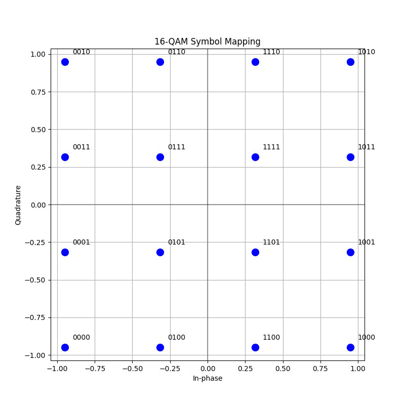
Understanding Symbol Mapping

Let’s visualize the bit mapping for 16-QAM

plt.figure(figsize=(8, 8))

# Create a sample pattern of all 16-QAM symbols
bit_patterns = []
symbols = []

for i in range(16):
    # Convert to 4-bit binary
    bits = [int(b) for b in format(i, "04b")]
    bit_patterns.append(bits)

    # Modulate just this one symbol
    symbol = qam16_mod(torch.tensor([bits]))
    symbols.append(symbol.item())

symbols_ct: torch.Tensor = torch.tensor(symbols, dtype=torch.complex64)

# Plot constellation with labels
plt.scatter(symbols_ct.real, symbols_ct.imag, color="blue", s=100)

# Add bit pattern labels to each point
for symbol, bits in zip(symbols_ct, bit_patterns):
    bit_str = "".join([str(b) for b in bits])
    plt.annotate(bit_str, (symbol.real + 0.05, symbol.imag + 0.05))

plt.grid(True)
plt.xlabel("In-phase")
plt.ylabel("Quadrature")
plt.title("16-QAM Symbol Mapping")
plt.axhline(y=0, color="k", linestyle="-", alpha=0.3)
plt.axvline(x=0, color="k", linestyle="-", alpha=0.3)
plt.axis("equal")
plt.show()

Performance in AWGN Channel

Compare BER for different QAM orders in AWGN

snr_db_range = np.arange(0, 31, 2)
ber_qam4 = []
ber_qam16 = []
ber_qam64 = []
ber_qam256 = []

# Initialize BER metric
ber_metric = BER()

for snr_db in snr_db_range:
    # Calculate noise power and create AWGN channel
    noise_power = snr_to_noise_power(1.0, snr_db)
    channel = AWGNChannel(avg_noise_power=noise_power)

    # 4-QAM transmission
    received_qam4 = channel(qam4_symbols)
    demod_bits_qam4 = qam4_demod(received_qam4)
    ber_qam4.append(ber_metric(demod_bits_qam4, qam4_bits).item())

    # 16-QAM transmission
    received_qam16 = channel(qam16_symbols)
    demod_bits_qam16 = qam16_demod(received_qam16)
    ber_qam16.append(ber_metric(demod_bits_qam16, qam16_bits).item())

    # 64-QAM transmission
    received_qam64 = channel(qam64_symbols)
    demod_bits_qam64 = qam64_demod(received_qam64)
    ber_qam64.append(ber_metric(demod_bits_qam64, qam64_bits).item())

    # 256-QAM transmission
    received_qam256 = channel(qam256_symbols)
    demod_bits_qam256 = qam256_demod(received_qam256)
    ber_qam256.append(ber_metric(demod_bits_qam256, qam256_bits).item())

# Plot BER vs SNR
plt.figure(figsize=(10, 6))
plt.semilogy(snr_db_range, ber_qam4, "b-", marker="o", label="4-QAM")
plt.semilogy(snr_db_range, ber_qam16, "g-", marker="s", label="16-QAM")
plt.semilogy(snr_db_range, ber_qam64, "r-", marker="^", label="64-QAM")
plt.semilogy(snr_db_range, ber_qam256, "m-", marker="*", label="256-QAM")

# Add approximate theoretical curves
snr_lin = 10 ** (snr_db_range / 10)
theoretical_ber_4qam = torch.erfc(torch.sqrt(torch.tensor(snr_lin))) / 2
theoretical_ber_16qam = 0.75 * torch.erfc(torch.sqrt(torch.tensor(snr_lin) / 5))
theoretical_ber_64qam = (7 / 12) * torch.erfc(torch.sqrt(torch.tensor(snr_lin) / 21))
theoretical_ber_256qam = (15 / 32) * torch.erfc(torch.sqrt(torch.tensor(snr_lin) / 85))

plt.semilogy(snr_db_range, theoretical_ber_4qam, "b--", alpha=0.5, label="4-QAM (Theory)")
plt.semilogy(snr_db_range, theoretical_ber_16qam, "g--", alpha=0.5, label="16-QAM (Theory)")
plt.semilogy(snr_db_range, theoretical_ber_64qam, "r--", alpha=0.5, label="64-QAM (Theory)")
plt.semilogy(snr_db_range, theoretical_ber_256qam, "m--", alpha=0.5, label="256-QAM (Theory)")

plt.grid(True)
plt.xlabel("SNR (dB)")
plt.ylabel("Bit Error Rate (BER)")
plt.title("BER Performance of QAM Modulations")
plt.legend()
plt.show()

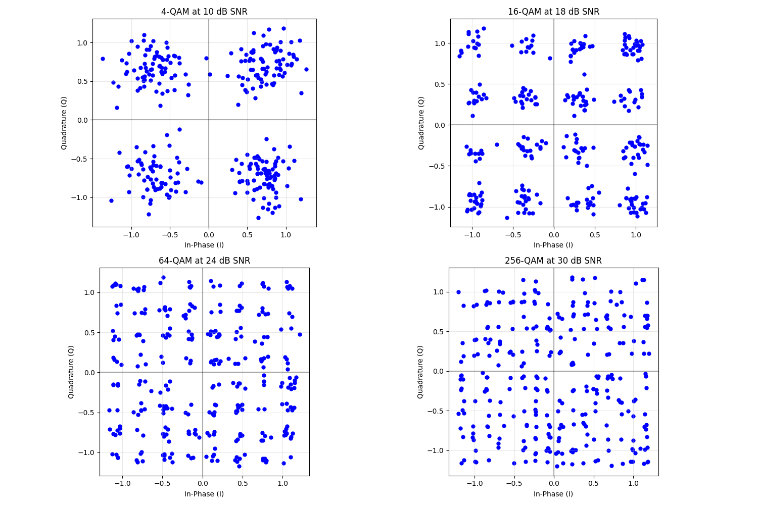
Effect of Noise on Constellations

Let’s visualize how noise affects the constellation diagrams at a fixed SNR

fig, axs = plt.subplots(2, 2, figsize=(15, 10))

# For each modulation, show the noisy constellation at the SNR needed for ~10^-3 BER
# These values are approximate based on the theoretical performance
snr_4qam = 10  # ~10 dB for 4-QAM to achieve 10^-3 BER
snr_16qam = 18  # ~18 dB for 16-QAM
snr_64qam = 24  # ~24 dB for 64-QAM
snr_256qam = 30  # ~30 dB for 256-QAM

# Generate test data with fewer symbols for clearer visualization
test_n_symbols = 300

# 4-QAM at 10 dB
test_bits = torch.randint(0, 2, (1, 2 * test_n_symbols))
test_symbols = qam4_mod(test_bits)
channel = AWGNChannel(avg_noise_power=snr_to_noise_power(1.0, snr_4qam))
received = channel(test_symbols)

plot_constellation(received.flatten(), title=f"4-QAM at {snr_4qam} dB SNR", marker=".", ax=axs[0, 0])
axs[0, 0].grid(True)

# 16-QAM at 18 dB
test_bits = torch.randint(0, 2, (1, 4 * test_n_symbols))
test_symbols = qam16_mod(test_bits)
channel = AWGNChannel(avg_noise_power=snr_to_noise_power(1.0, snr_16qam))
received = channel(test_symbols)

plot_constellation(received.flatten(), title=f"16-QAM at {snr_16qam} dB SNR", marker=".", ax=axs[0, 1])
axs[0, 1].grid(True)

# 64-QAM at 24 dB
test_bits = torch.randint(0, 2, (1, 6 * test_n_symbols))
test_symbols = qam64_mod(test_bits)
channel = AWGNChannel(avg_noise_power=snr_to_noise_power(1.0, snr_64qam))
received = channel(test_symbols)

plot_constellation(received.flatten(), title=f"64-QAM at {snr_64qam} dB SNR", marker=".", ax=axs[1, 0])
axs[1, 0].grid(True)

# 256-QAM at 30 dB
test_bits = torch.randint(0, 2, (1, 8 * test_n_symbols))
test_symbols = qam256_mod(test_bits)
channel = AWGNChannel(avg_noise_power=snr_to_noise_power(1.0, snr_256qam))
received = channel(test_symbols)

plot_constellation(received.flatten(), title=f"256-QAM at {snr_256qam} dB SNR", marker=".", ax=axs[1, 1])
axs[1, 1].grid(True)

plt.tight_layout()
plt.show()

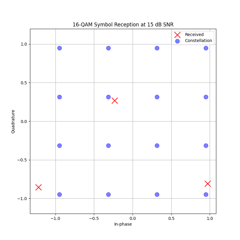
Hard vs. Soft Demodulation

Demonstrate difference between hard and soft demodulation for 16-QAM

demo_snr_db: int = 15
noise_power = snr_to_noise_power(1.0, demo_snr_db)
channel = AWGNChannel(avg_noise_power=noise_power)

# Generate a specific pattern that includes all four quadrants
test_bits = torch.tensor([[0, 0, 0, 0, 0, 1, 1, 1, 1, 0, 0, 0]])
test_symbols = qam16_mod(test_bits)

# Add noise
received = channel(test_symbols)

# Hard demodulation (without noise variance)
hard_bits = qam16_demod(received)

# Soft demodulation (with noise variance)
soft_llrs = qam16_demod(received, noise_var=noise_power)

# Print results
print("Original bits:", test_bits.numpy().flatten())
print("Hard decisions:", hard_bits.numpy().flatten().astype(int))
print("Soft LLRs:", soft_llrs.numpy().flatten())

# Plot the received symbol
plt.figure(figsize=(8, 8))
plt.scatter(received.real, received.imag, color="red", s=200, marker="x", label="Received")

# Plot the ideal constellation
# Get all 16 constellation points
all_symbols = qam16_mod(torch.tensor([[int(b) for b in format(i, "04b")] for i in range(16)]))
plt.scatter(all_symbols.real, all_symbols.imag, color="blue", s=100, alpha=0.5, marker="o", label="Constellation")

plt.grid(True)
plt.xlabel("In-phase")
plt.ylabel("Quadrature")
plt.title(f"16-QAM Symbol Reception at {demo_snr_db} dB SNR")
plt.legend()
plt.axis("equal")
plt.show()

Original bits: [0 0 0 0 0 1 1 1 1 0 0 0]
Hard decisions: [0 0 0 0 0 1 1 1 1 0 0 0]
Soft LLRs: [ 36.141632   11.74626    21.490463    4.420675    4.625809   -8.023301
  -5.358533   -7.290576  -26.20394     6.7774167  19.71098     3.5309343]

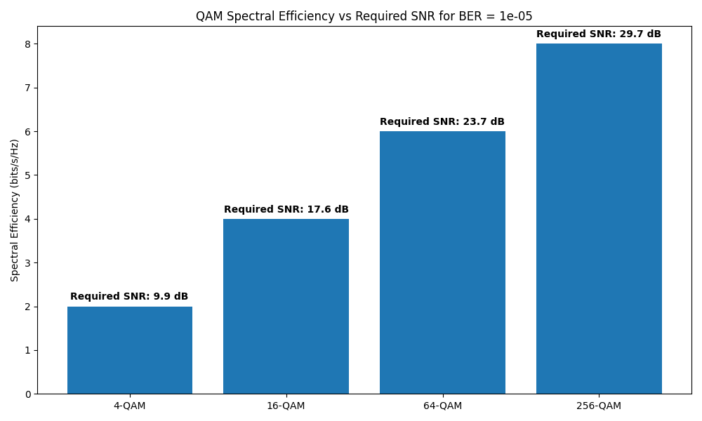
Efficiency vs. Performance Trade-off

Calculate approximate SNR required for different QAM orders at BER=10^-5

target_ber = 1e-5

# Interpolate required SNR from the theoretical curves
required_snr_4qam = np.interp(target_ber, theoretical_ber_4qam.numpy()[::-1], snr_db_range[::-1])
required_snr_16qam = np.interp(target_ber, theoretical_ber_16qam.numpy()[::-1], snr_db_range[::-1])
required_snr_64qam = np.interp(target_ber, theoretical_ber_64qam.numpy()[::-1], snr_db_range[::-1])
required_snr_256qam = np.interp(target_ber, theoretical_ber_256qam.numpy()[::-1], snr_db_range[::-1])

# Plot spectral efficiency vs required SNR
plt.figure(figsize=(10, 6))

# Create bar chart
modulations = ["4-QAM", "16-QAM", "64-QAM", "256-QAM"]
spectral_efficiencies = [2, 4, 6, 8]  # bits/s/Hz
required_snrs = [required_snr_4qam, required_snr_16qam, required_snr_64qam, required_snr_256qam]

bars = plt.bar(modulations, spectral_efficiencies)
plt.ylabel("Spectral Efficiency (bits/s/Hz)")
plt.title(f"QAM Spectral Efficiency vs Required SNR for BER = {target_ber}")

# Add SNR values on bars
for i, (bar, snr) in enumerate(zip(bars, required_snrs)):
    plt.text(i, bar.get_height() + 0.1, f"Required SNR: {snr:.1f} dB", ha="center", va="bottom", fontweight="bold")

plt.tight_layout()
plt.show()

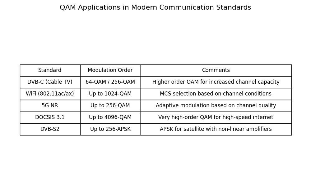
QAM Applications in Real-world Systems

This table shows examples of QAM usage in modern communication standards

plt.figure(figsize=(10, 6))
plt.axis("off")  # Turn off axis

standards = [
    "DVB-C (Cable TV)",
    "WiFi (802.11ac/ax)",
    "5G NR",
    "DOCSIS 3.1",
    "DVB-S2",
]

qam_orders = [
    "64-QAM / 256-QAM",
    "Up to 1024-QAM",
    "Up to 256-QAM",
    "Up to 4096-QAM",
    "Up to 256-APSK",
]

comments = [
    "Higher order QAM for increased channel capacity",
    "MCS selection based on channel conditions",
    "Adaptive modulation based on channel quality",
    "Very high-order QAM for high-speed internet",
    "APSK for satellite with non-linear amplifiers",
]

table_data = [["Standard", "Modulation Order", "Comments"]]
for std, order, comment in zip(standards, qam_orders, comments):
    table_data.append([std, order, comment])

# Create a table
table = plt.table(cellText=table_data, colWidths=[0.2, 0.2, 0.5], loc="center", cellLoc="center")
table.auto_set_font_size(False)
table.set_fontsize(12)
table.scale(1, 2)

plt.title("QAM Applications in Modern Communication Standards", fontsize=16, pad=20)
plt.tight_layout()
plt.show()

Conclusion

This example demonstrated:

1. Implementation of higher-order QAM modulation using Kaira

2. Visualization of constellation diagrams for different QAM orders

3. Symbol mapping for QAM schemes

4. BER performance comparison in AWGN channels

5. Performance requirements for different QAM orders

6. Hard vs. soft demodulation techniques

7. Real-world applications of QAM modulation

Key observations:

• QAM achieves high spectral efficiency by combining amplitude and phase modulation

• Higher-order QAM schemes provide more bits per symbol but require higher SNR

• Each QAM order approximately needs an additional 6dB SNR to maintain performance when doubling bits/symbol

• Modern communication systems use adaptive modulation to select the appropriate QAM order based on channel conditions

• Soft demodulation produces LLR values useful for soft-decision error correction coding