Composing Multiple Channel Effects

This example demonstrates how to compose multiple channel effects in Kaira to simulate complex transmission scenarios. In real communication systems, signals often pass through multiple channel impairments simultaneously, such as fading, phase noise, and additive noise. Kaira makes it easy to chain these effects together for realistic simulations.

import matplotlib.pyplot as plt

Imports and Setup

import numpy as np
import seaborn as sns
import torch

from kaira.channels import (
    AWGNChannel,
    BaseChannel,
    FlatFadingChannel,
    NonlinearChannel,
    PerfectChannel,
    PhaseNoiseChannel,
)

# Set random seed for reproducibility
torch.manual_seed(42)
np.random.seed(42)

Channel Composition in Kaira

Communication signals often traverse multiple channel impairments. For example: 1. RF signals experience nonlinear distortion in amplifiers 2. Then undergo fading due to multipath propagation 3. Experience phase noise in receiver oscillators 4. Finally, are corrupted by thermal AWGN noise

In Kaira, these effects can be chained by applying channels sequentially.

Generate a QAM Signal for Testing

Let’s create a 16-QAM constellation to illustrate channel effects.

def generate_qam_constellation(M=16):
    """Generate an M-QAM constellation (M must be a perfect square)."""
    # Verify M is a perfect square
    n = int(np.sqrt(M))
    if n**2 != M:
        raise ValueError("M must be a perfect square")

    # Create constellation points in a square grid
    x_coord = np.linspace(-1, 1, n)
    points = []

    for i in x_coord:
        for j in x_coord:
            points.append([i, j])

    # Convert to tensor and normalize power
    constellation = torch.tensor(points, dtype=torch.float32)
    power = torch.mean(torch.sum(constellation**2, dim=1))
    constellation = constellation / torch.sqrt(power)

    return constellation


# Generate QAM symbols
qam_points = generate_qam_constellation(16)
print(f"Generated {len(qam_points)} QAM constellation points")

# Create a batch of symbols by repeating each constellation point
num_per_point = 100
qam_symbols_list = []
for point in qam_points:
    qam_symbols_list.append(point.repeat(num_per_point, 1))

qam_symbols = torch.cat(qam_symbols_list, dim=0)
# Convert to complex form for easier processing
qam_complex = torch.complex(qam_symbols[:, 0], qam_symbols[:, 1])
# Reshape to add sequence dimension for FlatFadingChannel (batch_size, seq_length)
qam_complex = qam_complex.unsqueeze(1)
print(f"Created {len(qam_complex)} total QAM symbols with shape {qam_complex.shape}")

Generated 16 QAM constellation points
Created 1600 total QAM symbols with shape torch.Size([1600, 1])

Define Individual Channel Effects

Let’s create individual channels for each impairment type.

# 1. Nonlinear distortion (soft limiter / saturation)
def soft_limiter(x, alpha=1.2, saturation=0.8):
    """Soft limiter nonlinearity for complex signals."""
    magnitude = torch.abs(x)
    phase = torch.angle(x)

    # Apply nonlinear saturation to magnitude
    new_magnitude = saturation * torch.tanh(magnitude / saturation * alpha)

    # Reconstruct complex signal with original phase
    return new_magnitude * torch.exp(1j * phase)


nonlinear_channel = NonlinearChannel(nonlinear_fn=lambda x: soft_limiter(x, alpha=1.5, saturation=0.9), complex_mode="direct")

# 2. Fading channel (Rayleigh fading)
fading_channel = FlatFadingChannel(fading_type="rayleigh", coherence_time=50, snr_db=20)  # Symbols experience same fading across blocks  # High SNR to isolate fading effect

# 3. Phase noise channel
phase_noise_channel = PhaseNoiseChannel(phase_noise_std=0.1)  # 0.1 radians std dev

# 4. AWGN channel
awgn_channel = AWGNChannel(snr_db=15)  # 15 dB SNR

print("Created individual channel impairment models")

Created individual channel impairment models

Compose Channel Effects

Let’s create different channel compositions to see their combined effects. Note: order of application matters!

# Process signals through various channel combinations
with torch.no_grad():
    # Reference (perfect channel)
    perfect_output = qam_complex.clone()

    # Individual channel effects
    nonlinear_only = nonlinear_channel(qam_complex)
    fading_only = fading_channel(qam_complex)
    phase_noise_only = phase_noise_channel(qam_complex)
    awgn_only = awgn_channel(qam_complex)

    # Composite channels (realistic scenarios)
    # Scenario 1: Nonlinear → AWGN (e.g., satellite with nonlinear amplifier)
    nonlinear_awgn = awgn_channel(nonlinear_channel(qam_complex))

    # Scenario 2: Fading → AWGN (e.g., mobile wireless channel)
    fading_awgn = awgn_channel(fading_channel(qam_complex))

    # Scenario 3: Phase noise → AWGN (e.g., imperfect oscillator)
    phase_awgn = awgn_channel(phase_noise_channel(qam_complex))

    # Scenario 4: Full chain (all effects)
    full_chain = awgn_channel(phase_noise_channel(fading_channel(nonlinear_channel(qam_complex))))

print("Processed signals through various channel combinations")

Processed signals through various channel combinations

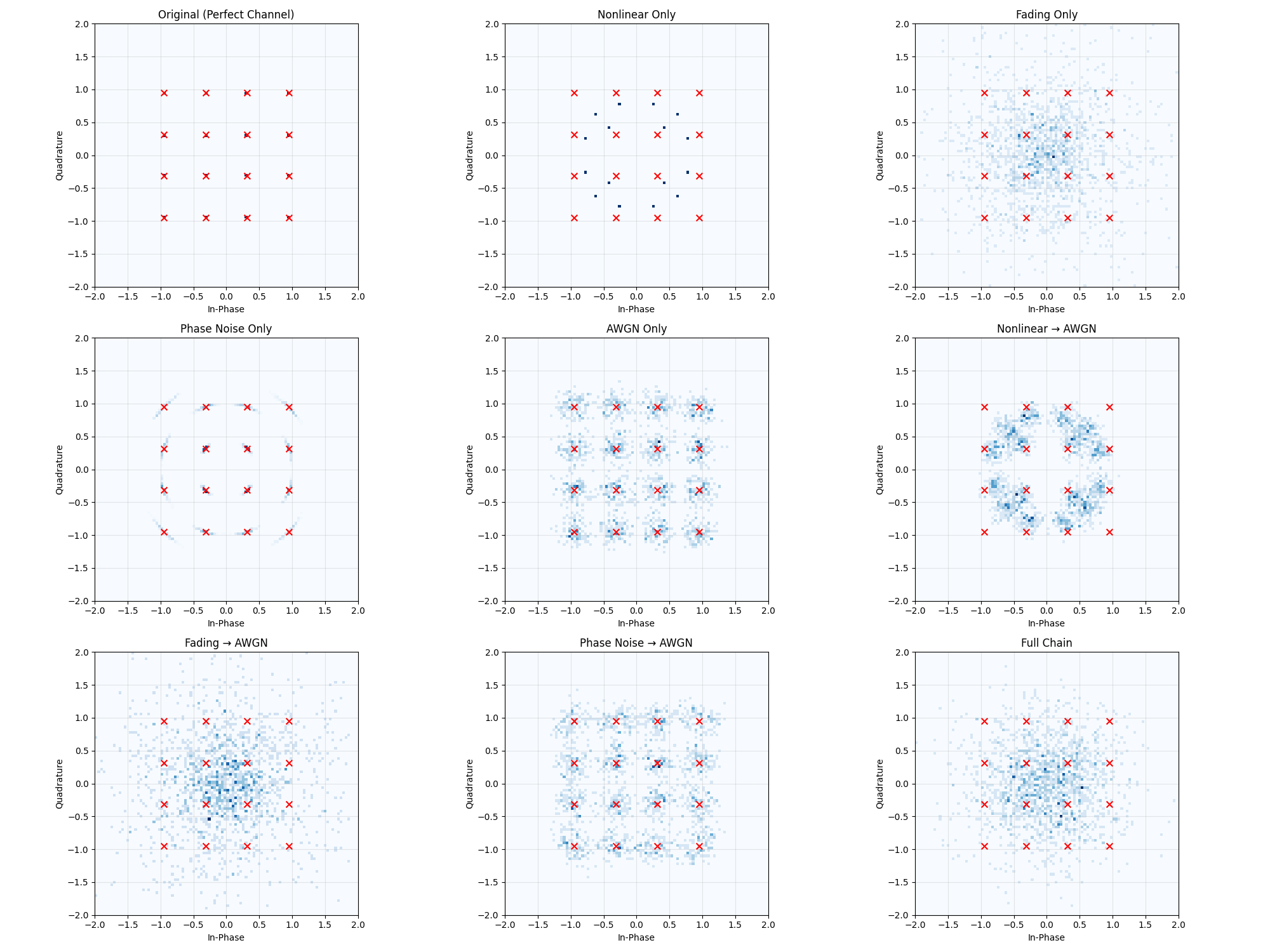
Visualize Channel Effects on Constellation

Let’s visualize how each channel and their combinations affect the constellation.

def plot_constellation(ax, symbols, title):
    """Plot a constellation diagram on the given axis."""
    # Squeeze out the sequence dimension if present
    if symbols.dim() > 1 and symbols.shape[1] == 1:
        symbols = symbols.squeeze(1)

    x = torch.real(symbols).cpu().numpy()
    y = torch.imag(symbols).cpu().numpy()

    # Create density-based scatter plot
    h = ax.hist2d(x, y, bins=100, range=[[-2, 2], [-2, 2]], cmap="Blues")

    # Plot original constellation points for reference
    orig_x = qam_points[:, 0].cpu().numpy()
    orig_y = qam_points[:, 1].cpu().numpy()
    ax.scatter(orig_x, orig_y, color="red", marker="x", s=50)

    ax.set_title(title)
    ax.set_xlabel("In-Phase")
    ax.set_ylabel("Quadrature")
    ax.grid(True, alpha=0.3)
    ax.set_xlim([-2, 2])
    ax.set_ylim([-2, 2])
    ax.set_aspect("equal")

    return h


# Create figure with constellation plots
plt.figure(figsize=(20, 15))

# Individual effects
plt.subplot(3, 3, 1)
plot_constellation(plt.gca(), perfect_output, "Original (Perfect Channel)")

plt.subplot(3, 3, 2)
plot_constellation(plt.gca(), nonlinear_only, "Nonlinear Only")

plt.subplot(3, 3, 3)
plot_constellation(plt.gca(), fading_only, "Fading Only")

plt.subplot(3, 3, 4)
plot_constellation(plt.gca(), phase_noise_only, "Phase Noise Only")

plt.subplot(3, 3, 5)
plot_constellation(plt.gca(), awgn_only, "AWGN Only")

# Composite effects
plt.subplot(3, 3, 6)
plot_constellation(plt.gca(), nonlinear_awgn, "Nonlinear → AWGN")

plt.subplot(3, 3, 7)
plot_constellation(plt.gca(), fading_awgn, "Fading → AWGN")

plt.subplot(3, 3, 8)
plot_constellation(plt.gca(), phase_awgn, "Phase Noise → AWGN")

plt.subplot(3, 3, 9)
plot_constellation(plt.gca(), full_chain, "Full Chain")

plt.tight_layout()
plt.show()

Analyze Symbol Error Rate

Let’s analyze how different channel impairments affect symbol error rate.

def calculate_ser(received, original_points):
    """Calculate Symbol Error Rate by finding closest constellation point."""
    # Convert inputs to numpy for processing
    received_np = torch.view_as_real(received).cpu().numpy()
    original_np = original_points.cpu().numpy()

    # Ground truth labels - which constellation point each symbol came from
    labels = np.repeat(np.arange(len(original_points)), num_per_point)

    # Detect closest constellation point for each received symbol
    detected = []
    for point in received_np:
        distances = np.sum((original_np - point) ** 2, axis=1)
        closest_idx = np.argmin(distances)
        detected.append(closest_idx)

    # Calculate error rate
    errors = np.array(detected) != labels
    ser = np.mean(errors)

    return ser


# Calculate SER for each channel scenario
channel_scenarios = [
    ("Perfect Channel", perfect_output),
    ("AWGN Only", awgn_only),
    ("Nonlinear Only", nonlinear_only),
    ("Phase Noise Only", phase_noise_only),
    ("Fading Only", fading_only),
    ("Nonlinear → AWGN", nonlinear_awgn),
    ("Phase Noise → AWGN", phase_awgn),
    ("Fading → AWGN", fading_awgn),
    ("Full Chain", full_chain),
]

# Calculate SER for each scenario
ser_results = []
for name, output in channel_scenarios:
    ser = calculate_ser(output, qam_points)
    ser_results.append((name, ser))
    print(f"{name}: SER = {ser:.4f}")

# Plot SER results
plt.figure(figsize=(12, 7))

# Extract data for plotting
scenario_names = [name for name, _ in ser_results]
ser_values = [ser for _, ser in ser_results]

# Create bar plot
bars = plt.bar(range(len(ser_results)), ser_values, width=0.7)

# Add value labels above bars
for i, v in enumerate(ser_values):
    if v > 0:
        plt.text(i, v + 0.01, f"{v:.3f}", ha="center")

# Customize plot
plt.xlabel("Channel Scenario")
plt.ylabel("Symbol Error Rate (SER)")
plt.title("Impact of Channel Impairments on Symbol Error Rate")
plt.xticks(range(len(ser_results)), scenario_names, rotation=45, ha="right")
plt.grid(True, axis="y", alpha=0.3)
plt.ylim(0, min(1.0, max(ser_values) * 1.2))  # Add some headroom for labels
plt.tight_layout()
plt.show()

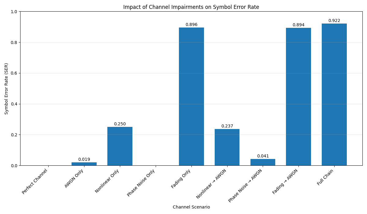
Perfect Channel: SER = 0.0000
AWGN Only: SER = 0.0194
Nonlinear Only: SER = 0.2500
Phase Noise Only: SER = 0.0000
Fading Only: SER = 0.8962
Nonlinear → AWGN: SER = 0.2369
Phase Noise → AWGN: SER = 0.0413
Fading → AWGN: SER = 0.8944
Full Chain: SER = 0.9219

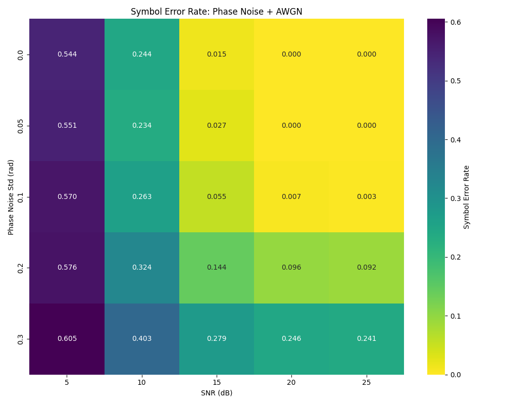
Sweep Parameter Combinations

Let’s explore how performance changes as we vary parameters of combined impairments. We’ll focus on phase noise + AWGN as an example.

# Define parameter ranges
phase_noise_levels = [0.0, 0.05, 0.1, 0.2, 0.3]
snr_db_levels = [5, 10, 15, 20, 25]

# Create grid of parameters
param_grid = []
for phase_std in phase_noise_levels:
    for snr_db in snr_db_levels:
        param_grid.append((phase_std, snr_db))

# Run composite channel for each parameter combination
ser_grid = []

for phase_std, snr_db in param_grid:
    # Create channels with these parameters
    if phase_std == 0.0:
        phase_ch = PerfectChannel()
    else:
        phase_ch = PhaseNoiseChannel(phase_noise_std=phase_std)

    awgn_ch = AWGNChannel(snr_db=snr_db)

    # Process through composite channel
    with torch.no_grad():
        output = awgn_ch(phase_ch(qam_complex))

    # Calculate SER
    ser = calculate_ser(output, qam_points)
    ser_grid.append((phase_std, snr_db, ser))
    print(f"Phase Noise: {phase_std:.2f} rad, SNR: {snr_db} dB, SER: {ser:.4f}")

Phase Noise: 0.00 rad, SNR: 5 dB, SER: 0.5444
Phase Noise: 0.00 rad, SNR: 10 dB, SER: 0.2437
Phase Noise: 0.00 rad, SNR: 15 dB, SER: 0.0150
Phase Noise: 0.00 rad, SNR: 20 dB, SER: 0.0000
Phase Noise: 0.00 rad, SNR: 25 dB, SER: 0.0000
Phase Noise: 0.05 rad, SNR: 5 dB, SER: 0.5506
Phase Noise: 0.05 rad, SNR: 10 dB, SER: 0.2344
Phase Noise: 0.05 rad, SNR: 15 dB, SER: 0.0269
Phase Noise: 0.05 rad, SNR: 20 dB, SER: 0.0000
Phase Noise: 0.05 rad, SNR: 25 dB, SER: 0.0000
Phase Noise: 0.10 rad, SNR: 5 dB, SER: 0.5700
Phase Noise: 0.10 rad, SNR: 10 dB, SER: 0.2625
Phase Noise: 0.10 rad, SNR: 15 dB, SER: 0.0550
Phase Noise: 0.10 rad, SNR: 20 dB, SER: 0.0069
Phase Noise: 0.10 rad, SNR: 25 dB, SER: 0.0025
Phase Noise: 0.20 rad, SNR: 5 dB, SER: 0.5756
Phase Noise: 0.20 rad, SNR: 10 dB, SER: 0.3244
Phase Noise: 0.20 rad, SNR: 15 dB, SER: 0.1437
Phase Noise: 0.20 rad, SNR: 20 dB, SER: 0.0963
Phase Noise: 0.20 rad, SNR: 25 dB, SER: 0.0919
Phase Noise: 0.30 rad, SNR: 5 dB, SER: 0.6050
Phase Noise: 0.30 rad, SNR: 10 dB, SER: 0.4031
Phase Noise: 0.30 rad, SNR: 15 dB, SER: 0.2787
Phase Noise: 0.30 rad, SNR: 20 dB, SER: 0.2456
Phase Noise: 0.30 rad, SNR: 25 dB, SER: 0.2406

Create a heatmap of SER vs. parameters

# Prepare data for heatmap
ser_matrix = np.zeros((len(phase_noise_levels), len(snr_db_levels)))
for i, phase_std in enumerate(phase_noise_levels):
    for j, snr_db in enumerate(snr_db_levels):
        # Find matching grid point
        for p, s, ser in ser_grid:
            if p == phase_std and s == snr_db:
                ser_matrix[i, j] = ser
                break

plt.figure(figsize=(10, 8))

# Create heatmap
ax = sns.heatmap(ser_matrix, annot=True, fmt=".3f", cmap="viridis_r", xticklabels=[str(x) for x in snr_db_levels], yticklabels=[str(y) for y in phase_noise_levels])

plt.xlabel("SNR (dB)")
plt.ylabel("Phase Noise Std (rad)")
plt.title("Symbol Error Rate: Phase Noise + AWGN")
cbar = ax.collections[0].colorbar
if cbar is not None:
    cbar.set_label("Symbol Error Rate")
plt.tight_layout()
plt.show()

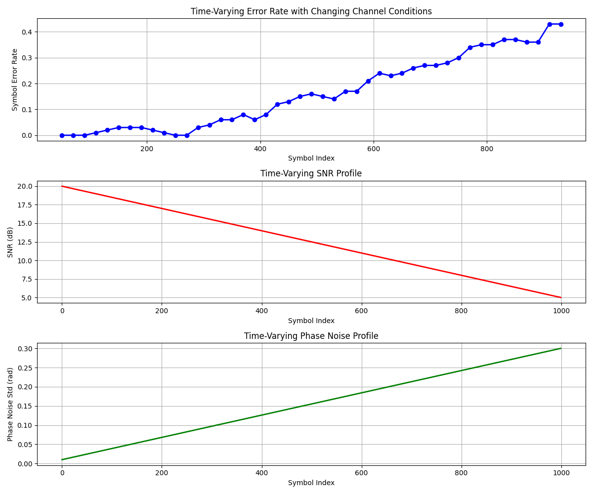
Time-Varying Channel Example

Let’s demonstrate a time-varying channel where parameters change over time. This simulates scenarios like mobile communications with changing conditions.

# Generate a longer sequence of QAM symbols
seq_length = 1000
symbol_indices = torch.randint(0, len(qam_points), (seq_length,))
symbols = qam_points[symbol_indices]
symbols_complex = torch.complex(symbols[:, 0], symbols[:, 1])


# Create a time-varying channel function
def time_varying_channel(x, time_axis):
    """Apply time-varying channel effects to the input signal."""
    # Get sequence length
    seq_len = len(x)

    # Create time-varying SNR profile (moving from good to poor conditions)
    snr_profile = torch.linspace(20, 5, seq_len)  # SNR from 20dB to 5dB

    # Create time-varying phase noise profile
    phase_noise_profile = torch.linspace(0.01, 0.3, seq_len)  # Increasing phase noise

    # Process each symbol individually with its own parameters
    output = torch.zeros_like(x)

    for i in range(seq_len):
        # Get current parameters
        current_snr = snr_profile[i].item()
        current_phase_std = phase_noise_profile[i].item()

        # Create channels with current parameters
        phase_ch = PhaseNoiseChannel(phase_noise_std=current_phase_std)
        awgn_ch = AWGNChannel(snr_db=current_snr)

        # Apply to current symbol
        with torch.no_grad():
            symbol = x[i : i + 1]  # Keep batch dimension
            output[i] = awgn_ch(phase_ch(symbol))[0]

    return output


# Apply time-varying channel
time_axis = np.arange(seq_length)
with torch.no_grad():
    time_varying_output = time_varying_channel(symbols_complex, time_axis)

Analyze Time-Varying Effects

Let’s analyze how performance varies over time with changing conditions.

# Calculate error rate in sliding windows
window_size = 100
stride = 20
windows = []
window_ser = []

for i in range(0, seq_length - window_size, stride):
    # Extract current window
    window_output = time_varying_output[i : i + window_size]
    window_indices = symbol_indices[i : i + window_size]

    # Calculate error rate in this window
    detected_indices = []
    for symbol in window_output:
        # Convert to real+imag components
        point = torch.tensor([torch.real(symbol).item(), torch.imag(symbol).item()])

        # Find closest constellation point
        distances = torch.sum((qam_points - point) ** 2, dim=1)
        detected_idx = torch.argmin(distances).item()
        detected_indices.append(detected_idx)

    # Calculate SER in window
    errors = np.array(detected_indices) != window_indices.numpy()
    window_error_rate = np.mean(errors)

    # Store window center and SER
    window_center = i + window_size // 2
    windows.append(window_center)
    window_ser.append(window_error_rate)

Plot time-varying SER

plt.figure(figsize=(12, 10))

# Create time-varying parameter profiles for plotting
time_points = np.linspace(0, seq_length - 1, 100)
snr_profile = 20 - 15 * (time_points / (seq_length - 1))
phase_profile = 0.01 + 0.29 * (time_points / (seq_length - 1))

# Plot SER vs. time
plt.subplot(3, 1, 1)
plt.plot(windows, window_ser, "bo-", linewidth=2)
plt.grid(True)
plt.xlabel("Symbol Index")
plt.ylabel("Symbol Error Rate")
plt.title("Time-Varying Error Rate with Changing Channel Conditions")

# Plot SNR profile
plt.subplot(3, 1, 2)
plt.plot(time_points, snr_profile, "r-", linewidth=2)
plt.grid(True)
plt.xlabel("Symbol Index")
plt.ylabel("SNR (dB)")
plt.title("Time-Varying SNR Profile")

# Plot phase noise profile
plt.subplot(3, 1, 3)
plt.plot(time_points, phase_profile, "g-", linewidth=2)
plt.grid(True)
plt.xlabel("Symbol Index")
plt.ylabel("Phase Noise Std (rad)")
plt.title("Time-Varying Phase Noise Profile")

plt.tight_layout()
plt.show()

Creating a Custom Composite Channel Class

For repeated use, you can create a custom composite channel class.

class SatelliteChannel(BaseChannel):
    """A composite channel model for satellite communications.

    This model chains together typical impairments found in satellite links:
    1. Nonlinear amplifier distortion (TWT/HPA)
    2. Phase noise from oscillator imperfections
    3. AWGN from thermal noise
    """

    def __init__(self, nonlinearity_factor=1.5, phase_noise_std=0.1, snr_db=15):
        """Initialize with desired parameters for each component."""
        super().__init__()

        # Create component channels
        self.nonlinear_ch = NonlinearChannel(nonlinear_fn=lambda x: soft_limiter(x, alpha=nonlinearity_factor, saturation=0.9), complex_mode="direct")

        self.phase_noise_ch = PhaseNoiseChannel(phase_noise_std=phase_noise_std)
        self.awgn_ch = AWGNChannel(snr_db=snr_db)

    def forward(self, x):
        """Apply the full chain of channel effects."""
        # Apply each component in sequence
        y = self.nonlinear_ch(x)
        y = self.phase_noise_ch(y)
        y = self.awgn_ch(y)
        return y

    def get_config(self):
        """Return the configuration parameters."""
        return {"nonlinear_ch": self.nonlinear_ch.get_config(), "phase_noise_ch": self.phase_noise_ch.get_config(), "awgn_ch": self.awgn_ch.get_config()}


# Create satellite channel with default parameters
satellite_channel = SatelliteChannel()

# Process signals through the custom composite channel
with torch.no_grad():
    satellite_output = satellite_channel(qam_complex)

# Calculate SER
satellite_ser = calculate_ser(satellite_output, qam_points)
print(f"Satellite Channel SER: {satellite_ser:.4f}")

# Visualize constellation
plt.figure(figsize=(10, 8))
plot_constellation(plt.gca(), satellite_output, "Satellite Channel (Composite)")
plt.tight_layout()
plt.show()

Satellite Channel SER: 0.2556

Conclusion

This example demonstrates several key aspects of channel composition in Kaira:

• Individual channel effects can be combined in sequence to model complex real-world communication scenarios

• The order of channel effects matters and should reflect the physical signal path (e.g., nonlinear distortion at transmitter, fading during propagation, phase noise and AWGN at receiver)

• Combined effects often result in more severe performance degradation than individual impairments

• Parameter interactions between channel effects can be complex and are easily explored using Kaira’s modular design

• Custom composite channels can be created for reusable, complex channel models

By composing channel effects, Kaira enables realistic simulation of communication systems, allowing researchers and engineers to evaluate performance under conditions that closely match real-world scenarios.