Impulsive Noise with Laplacian Channel

This example demonstrates the LaplacianChannel in Kaira, which models channels with impulsive noise that follows the Laplacian distribution. Unlike Gaussian noise, Laplacian noise has heavier tails, making it suitable for modeling environments with occasional large noise spikes.

import matplotlib.pyplot as plt

Imports and Setup

import numpy as np
import seaborn as sns
import torch

from kaira.channels import AWGNChannel, LaplacianChannel
from kaira.utils import snr_to_noise_power

# Set random seed for reproducibility
torch.manual_seed(42)
np.random.seed(42)

Generate Sample Signal

Let’s create a sample signal to test our noise models.

# Generate time points
t = np.linspace(0, 1, 1000)
# Create a multi-tone signal (sum of several sinusoids)
signal = 0.5 * np.sin(2 * np.pi * 3 * t) + 0.3 * np.sin(2 * np.pi * 7 * t) + 0.2 * np.cos(2 * np.pi * 11 * t)

# Convert to torch tensor
input_signal = torch.from_numpy(signal).float().reshape(1, -1)
print(f"Input signal shape: {input_signal.shape}")

Input signal shape: torch.Size([1, 1000])

Create Channels with Different Noise Distributions

We’ll compare Gaussian noise (AWGNChannel) with Laplacian noise at equivalent SNR levels.

# Define SNR levels in dB
snr_levels_db = [20, 10, 0]
signal_power = np.mean(signal**2)

# Create channels for comparison
channels = []
for snr_db in snr_levels_db:
    # Calculate noise power from SNR
    noise_power = snr_to_noise_power(signal_power, snr_db)

    # Create AWGN channel (Gaussian noise)
    awgn_channel = AWGNChannel(avg_noise_power=noise_power)

    # Create Laplacian channel (for impulsive noise)
    laplacian_channel = LaplacianChannel(avg_noise_power=noise_power)

    channels.append((snr_db, awgn_channel, laplacian_channel))
    print(f"Created channels with SNR: {snr_db} dB (noise power: {noise_power:.6f})")

Created channels with SNR: 20 dB (noise power: 0.001899)
Created channels with SNR: 10 dB (noise power: 0.018985)
Created channels with SNR: 0 dB (noise power: 0.189850)

Pass Signal Through Channels

Now we’ll pass our signal through each channel and collect the outputs.

awgn_outputs = []
laplacian_outputs = []

for snr_db, awgn_channel, laplacian_channel in channels:
    with torch.no_grad():
        # Pass through AWGN channel
        awgn_output = awgn_channel(input_signal)

        # Pass through Laplacian channel
        laplacian_output = laplacian_channel(input_signal)

    # Store results
    awgn_outputs.append((snr_db, awgn_output.numpy().flatten()))
    laplacian_outputs.append((snr_db, laplacian_output.numpy().flatten()))

Visualize Noise Distribution Differences

Let’s compare the effect of Gaussian vs. Laplacian noise on our signal.

plt.figure(figsize=(15, 12))

# Plot the original signal first
plt.subplot(len(snr_levels_db) + 1, 2, 1)
plt.plot(t, signal, "k-", linewidth=1.5)
plt.title("Original Signal")
plt.grid(True)
plt.ylabel("Amplitude")
plt.xlim([0, 1])

# Empty plot for alignment
plt.subplot(len(snr_levels_db) + 1, 2, 2)
plt.axis("off")

# Plot each noisy signal
for i, (snr_db, awgn_output, laplacian_output) in enumerate(zip([level for level, _, _ in channels], [output for _, output in awgn_outputs], [output for _, output in laplacian_outputs])):
    # Plot AWGN channel output
    plt.subplot(len(snr_levels_db) + 1, 2, 2 * i + 3)
    plt.plot(t, awgn_output, "b-", alpha=0.8)
    plt.title(f"AWGN Channel (SNR = {snr_db} dB)")
    plt.grid(True)
    plt.ylabel("Amplitude")
    plt.xlim([0, 1])

    # Plot Laplacian channel output
    plt.subplot(len(snr_levels_db) + 1, 2, 2 * i + 4)
    plt.plot(t, laplacian_output, "r-", alpha=0.8)
    plt.title(f"Laplacian Channel (SNR = {snr_db} dB)")
    plt.grid(True)
    plt.ylabel("Amplitude")
    plt.xlim([0, 1])

plt.tight_layout()
plt.show()

Analyze Noise Distribution

To better understand the difference between Gaussian and Laplacian noise, let’s extract the noise components and visualize their distributions.

def extract_noise(noisy_signal, original_signal):
    """Extract the noise component from a noisy signal."""
    return noisy_signal - original_signal


# Choose a specific SNR level for analysis
snr_idx = 1  # Using the middle SNR level
snr_db = snr_levels_db[snr_idx]
awgn_noise = extract_noise(awgn_outputs[snr_idx][1], signal)
laplacian_noise = extract_noise(laplacian_outputs[snr_idx][1], signal)

plt.figure(figsize=(14, 6))

# Plot noise histograms
plt.subplot(1, 2, 1)
sns.histplot(awgn_noise, kde=True, stat="density", label="Gaussian Noise", color="blue", alpha=0.6)
sns.histplot(laplacian_noise, kde=True, stat="density", label="Laplacian Noise", color="red", alpha=0.6)

# Add theoretical PDF curves
x = np.linspace(-1, 1, 1000)
# Standard deviation of extracted noise
gaussian_std = np.std(awgn_noise)
laplacian_scale = np.std(laplacian_noise) / np.sqrt(2)  # Relation between std and scale for Laplacian

# Gaussian PDF
gaussian_pdf = (1 / (gaussian_std * np.sqrt(2 * np.pi))) * np.exp(-0.5 * (x / gaussian_std) ** 2)
plt.plot(x, gaussian_pdf, "b-", linewidth=2, label="Gaussian PDF")

# Laplacian PDF
laplacian_pdf = (1 / (2 * laplacian_scale)) * np.exp(-np.abs(x) / laplacian_scale)
plt.plot(x, laplacian_pdf, "r-", linewidth=2, label="Laplacian PDF")

plt.grid(True)
plt.title(f"Noise Distribution Comparison (SNR = {snr_db} dB)")
plt.xlabel("Amplitude")
plt.ylabel("Density")
plt.legend()
plt.xlim([-0.5, 0.5])

# Plot in log scale to highlight the tails
plt.subplot(1, 2, 2)
plt.semilogy(np.sort(np.abs(awgn_noise)), np.linspace(1, 0, len(awgn_noise)), "b-", linewidth=2, label="Gaussian Noise")
plt.semilogy(np.sort(np.abs(laplacian_noise)), np.linspace(1, 0, len(laplacian_noise)), "r-", linewidth=2, label="Laplacian Noise")
plt.grid(True)
plt.title("CCDF of Absolute Noise Value")
plt.xlabel("Absolute Noise Amplitude")
plt.ylabel("Probability (Noise > x)")
plt.legend()

plt.tight_layout()
plt.show()

Impact on Error Metrics

Let’s analyze how the different noise distributions impact common error metrics.

plt.figure(figsize=(10, 6))

# Calculate MSE for each SNR level
awgn_mse = []
laplacian_mse = []
awgn_peak_error = []
laplacian_peak_error = []

for (snr1, awgn_output), (snr2, laplacian_output) in zip(awgn_outputs, laplacian_outputs):
    assert snr1 == snr2, "SNR levels should match"

    # Calculate MSE
    awgn_mse.append(np.mean((signal - awgn_output) ** 2))
    laplacian_mse.append(np.mean((signal - laplacian_output) ** 2))

    # Calculate peak error (max absolute error)
    awgn_peak_error.append(np.max(np.abs(signal - awgn_output)))
    laplacian_peak_error.append(np.max(np.abs(signal - laplacian_output)))

# Plot MSE vs. SNR
plt.subplot(1, 2, 1)
plt.plot(snr_levels_db, awgn_mse, "bo-", linewidth=2, label="AWGN Channel")
plt.plot(snr_levels_db, laplacian_mse, "ro-", linewidth=2, label="Laplacian Channel")
plt.grid(True)
plt.title("Mean Squared Error vs. SNR")
plt.xlabel("SNR (dB)")
plt.ylabel("MSE")
plt.legend()
plt.yscale("log")

# Plot Peak Error vs. SNR
plt.subplot(1, 2, 2)
plt.plot(snr_levels_db, awgn_peak_error, "bs-", linewidth=2, label="AWGN Channel")
plt.plot(snr_levels_db, laplacian_peak_error, "rs-", linewidth=2, label="Laplacian Channel")
plt.grid(True)
plt.title("Peak Error vs. SNR")
plt.xlabel("SNR (dB)")
plt.ylabel("Peak Error")
plt.legend()
plt.yscale("log")

plt.tight_layout()
plt.show()

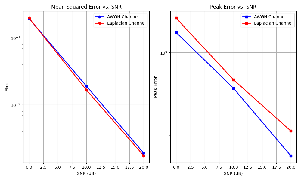
Conclusion

This example demonstrates the key differences between Gaussian noise (AWGN) and Laplacian noise when applied to signals:

• Laplacian noise has heavier tails than Gaussian noise, resulting in more frequent large-magnitude noise spikes

• While both channels can be configured for the same average noise power (SNR), the Laplacian channel typically produces higher peak errors

• Laplacian noise better models impulsive disturbances that occur in certain communication environments, such as urban settings with electrical interference

The choice between these noise models depends on the specific communication environment being simulated. When occasional large noise spikes are expected, the LaplacianChannel provides a more realistic model than the standard AWGNChannel.