Nonlinear Channel Distortion Effects

This example demonstrates the NonlinearChannel in Kaira, which allows modeling various nonlinear signal distortions commonly encountered in communication systems. Nonlinearities occur in many components such as amplifiers, mixers, and converters, and can significantly impact system performance.

import matplotlib.pyplot as plt

Imports and Setup

import numpy as np
import torch
from scipy import signal

from kaira.channels import AWGNChannel, NonlinearChannel, PerfectChannel
from kaira.metrics.signal import SymbolErrorRate
from kaira.modulations import QAMModulator

# Set random seed for reproducibility
torch.manual_seed(42)
np.random.seed(42)

Define Nonlinear Transfer Functions

We’ll define several common nonlinear distortion functions.

def soft_clipping(x, alpha=1.0):
    """Soft clipping/saturation nonlinearity using tanh."""
    return torch.tanh(alpha * x)


def hard_clipping(x, threshold=0.8):
    """Hard clipping at specified threshold value."""
    return torch.clamp(x, min=-threshold, max=threshold)


def saleh_amplitude(x, alpha_a=2.0, beta_a=1.0):
    """Saleh model for amplitude AM/AM distortion (commonly used for TWT amplifiers)."""
    r = torch.abs(x)
    return (alpha_a * r) / (1.0 + beta_a * r**2)


def saleh_phase(x, alpha_p=2.0, beta_p=1.0):
    """Saleh model for AM/PM distortion."""
    r = torch.abs(x)
    return (alpha_p * r**2) / (1.0 + beta_p * r**2)


def saleh_model(x, alpha_a=2.0, beta_a=1.0, alpha_p=2.0, beta_p=1.0):
    """Complete Saleh model (AM/AM and AM/PM)."""
    r = torch.abs(x)
    theta = torch.angle(x)

    # AM/AM distortion
    A = (alpha_a * r) / (1.0 + beta_a * r**2)

    # AM/PM distortion
    phi = (alpha_p * r**2) / (1.0 + beta_p * r**2)

    # Reconstruct signal
    return A * torch.exp(1j * (theta + phi))


def polynomial_nonlinearity(x, coeffs=[1.0, 0.2, -0.1]):
    """Polynomial nonlinearity (odd-order for real signals)."""
    result = torch.zeros_like(x)
    for i, coeff in enumerate(coeffs):
        result += coeff * (x ** (i + 1))
    return result

Generate Test Signals

Let’s create test signals to observe nonlinear distortion effects.

# Generate time points
t = np.linspace(0, 1, 1000)

# Generate a single-tone signal
freq_single = 5  # Hz
signal_single = np.sin(2 * np.pi * freq_single * t)

# Generate a two-tone signal
freq1 = 5  # Hz
freq2 = 7  # Hz
signal_two_tone = 0.5 * np.sin(2 * np.pi * freq1 * t) + 0.5 * np.sin(2 * np.pi * freq2 * t)

# Convert to torch tensors
input_single = torch.from_numpy(signal_single).float().reshape(1, -1)
input_two_tone = torch.from_numpy(signal_two_tone).float().reshape(1, -1)

print("Generated single-tone and two-tone test signals")

Generated single-tone and two-tone test signals

Apply Different Nonlinear Distortions

Now we’ll pass our test signals through various nonlinear channels.

# Create different nonlinear channels
nonlinear_channels = [
    ("Linear (Reference)", PerfectChannel()),
    ("Soft Clipping", NonlinearChannel(lambda x: soft_clipping(x, alpha=2.0))),
    ("Hard Clipping", NonlinearChannel(lambda x: hard_clipping(x, threshold=0.5))),
    ("Polynomial", NonlinearChannel(lambda x: polynomial_nonlinearity(x, coeffs=[1.0, 0.0, -0.25]))),
]

# Process signals through each channel
single_tone_outputs = []
two_tone_outputs = []

for name, channel in nonlinear_channels:
    with torch.no_grad():
        # Process single-tone signal
        single_output = channel(input_single)

        # Process two-tone signal
        two_output = channel(input_two_tone)

    # Store results
    single_tone_outputs.append((name, single_output.numpy().flatten()))
    two_tone_outputs.append((name, two_output.numpy().flatten()))
    print(f"Processed signals through {name} channel")

Processed signals through Linear (Reference) channel
Processed signals through Soft Clipping channel
Processed signals through Hard Clipping channel
Processed signals through Polynomial channel

Visualize Time-Domain Distortion Effects

Let’s visualize how nonlinearities affect signals in the time domain.

plt.figure(figsize=(15, 10))

# Plot single-tone signal results
plt.subplot(2, 1, 1)
for i, (name, output) in enumerate(single_tone_outputs):
    plt.plot(t, output, label=name, alpha=0.7, linewidth=2)

plt.grid(True)
plt.title("Nonlinear Distortion Effects on Single-Tone Signal")
plt.xlabel("Time (s)")
plt.ylabel("Amplitude")
plt.legend()

# Plot two-tone signal results
plt.subplot(2, 1, 2)
for i, (name, output) in enumerate(two_tone_outputs):
    plt.plot(t, output, label=name, alpha=0.7, linewidth=2)

plt.grid(True)
plt.title("Nonlinear Distortion Effects on Two-Tone Signal")
plt.xlabel("Time (s)")
plt.ylabel("Amplitude")
plt.legend()

plt.tight_layout()
plt.show()

Frequency-Domain Analysis

Let’s analyze the spectral effects of nonlinear distortion.

def calculate_spectrum(signal_data, fs=1000):
    """Calculate the power spectrum of a signal."""
    # Use Welch's method for better spectral estimation
    f, Pxx = signal.welch(signal_data, fs=fs, nperseg=512, scaling="spectrum", return_onesided=True)
    # Convert to dB
    Pxx_db = 10 * np.log10(Pxx + 1e-10)  # Adding small value to avoid log(0)
    return f, Pxx_db


plt.figure(figsize=(15, 10))

# Calculate and plot spectrum for single-tone signals
plt.subplot(2, 1, 1)
for name, output in single_tone_outputs:
    f, Pxx = calculate_spectrum(output)
    plt.plot(f, Pxx, label=name, alpha=0.7, linewidth=2)

plt.grid(True)
plt.title("Spectrum of Single-Tone Signal after Nonlinear Distortion")
plt.xlabel("Frequency (Hz)")
plt.ylabel("Power Spectrum (dB)")
plt.xlim([0, 30])  # Focus on the main frequency range
plt.legend()

# Calculate and plot spectrum for two-tone signals
plt.subplot(2, 1, 2)
for name, output in two_tone_outputs:
    f, Pxx = calculate_spectrum(output)
    plt.plot(f, Pxx, label=name, alpha=0.7, linewidth=2)

plt.grid(True)
plt.title("Spectrum of Two-Tone Signal after Nonlinear Distortion")
plt.xlabel("Frequency (Hz)")
plt.ylabel("Power Spectrum (dB)")
plt.xlim([0, 30])  # Focus on the main frequency range
plt.legend()

plt.tight_layout()
plt.show()

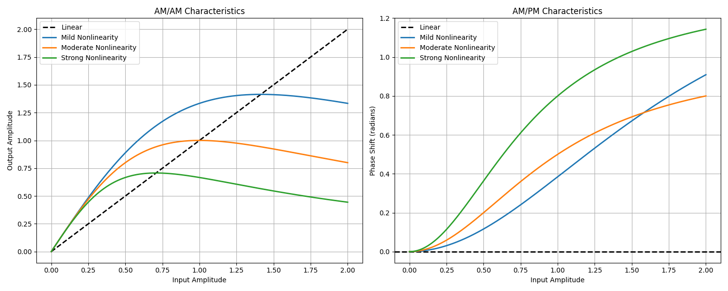
AM/AM and AM/PM Characteristics

Now let’s examine the amplitude and phase distortion characteristics of the Saleh model commonly used for modeling power amplifiers.

# Create an input signal with varying amplitude for testing
test_amplitude = torch.linspace(0, 2, 1000)
# Use torch.complex() to create complex tensors instead of torch.exp with Python complex numbers
test_complex = torch.complex(test_amplitude, torch.zeros_like(test_amplitude))  # Complex signal with zero phase

# Create Saleh model nonlinear channel with different parameters
saleh_channels = [
    ("Mild Nonlinearity", NonlinearChannel(lambda x: saleh_model(x, alpha_a=2.0, beta_a=0.5, alpha_p=0.5, beta_p=0.3), complex_mode="direct")),
    ("Moderate Nonlinearity", NonlinearChannel(lambda x: saleh_model(x, alpha_a=2.0, beta_a=1.0, alpha_p=1.0, beta_p=1.0), complex_mode="direct")),
    ("Strong Nonlinearity", NonlinearChannel(lambda x: saleh_model(x, alpha_a=2.0, beta_a=2.0, alpha_p=2.0, beta_p=1.5), complex_mode="direct")),
]

# Process test signal through saleh channels
saleh_outputs = []

for name, channel in saleh_channels:
    with torch.no_grad():
        output = channel(test_complex)

    # Extract amplitude and phase
    output_amp = torch.abs(output).numpy()
    output_phase = torch.angle(output).numpy()

    saleh_outputs.append((name, output_amp, output_phase))
    print(f"Processed signal through {name} Saleh channel")

# Plot AM/AM and AM/PM characteristics
plt.figure(figsize=(15, 6))

# AM/AM (amplitude) characteristics
plt.subplot(1, 2, 1)
plt.plot(test_amplitude.numpy(), test_amplitude.numpy(), "k--", label="Linear", linewidth=2)

for name, amp, phase in saleh_outputs:
    plt.plot(test_amplitude.numpy(), amp, label=name, linewidth=2)

plt.grid(True)
plt.title("AM/AM Characteristics")
plt.xlabel("Input Amplitude")
plt.ylabel("Output Amplitude")
plt.legend()

# AM/PM (phase) characteristics
plt.subplot(1, 2, 2)
plt.axhline(y=0, color="k", linestyle="--", label="Linear", linewidth=2)

for name, amp, phase in saleh_outputs:
    plt.plot(test_amplitude.numpy(), phase, label=name, linewidth=2)

plt.grid(True)
plt.title("AM/PM Characteristics")
plt.xlabel("Input Amplitude")
plt.ylabel("Phase Shift (radians)")
plt.legend()

plt.tight_layout()
plt.show()

Processed signal through Mild Nonlinearity Saleh channel
Processed signal through Moderate Nonlinearity Saleh channel
Processed signal through Strong Nonlinearity Saleh channel

Effect of Nonlinearities on Digital Modulation

Let’s examine how nonlinear distortion affects a 16-QAM constellation.

# Use Kaira's QAMModulator to generate QAM symbols
qam_modulator = QAMModulator(16)

# Generate random bits for 10000 random 16-QAM symbols
n_symbols = 10000
bits_per_symbol = 4  # 16-QAM uses 4 bits per symbol
random_bits = torch.randint(0, 2, (1, n_symbols * bits_per_symbol)).float()

# Modulate bits to symbols
with torch.no_grad():
    qam_symbols = qam_modulator(random_bits)

# Create different nonlinear channels for constellation test
qam_channels = [
    ("Linear", PerfectChannel()),
    ("Mild Nonlinearity", NonlinearChannel(lambda x: saleh_model(x, alpha_a=4.0, beta_a=0.1, alpha_p=0.5, beta_p=0.1), complex_mode="direct")),
    ("Strong Nonlinearity", NonlinearChannel(lambda x: saleh_model(x, alpha_a=3.5, beta_a=0.5, alpha_p=1.5, beta_p=0.5), complex_mode="direct")),
]

# Add AWGN after nonlinear distortion
awgn_channel = AWGNChannel(avg_noise_power=0.01)

# Create a Kaira Symbol Error Rate metric
ser_metric = SymbolErrorRate()

# Process QAM symbols through each channel
qam_outputs = []
ser_results = []

# Get the constellation points for later reference
constellation_points = qam_modulator.constellation

# Create labels for symbols (for later use in SER calculation)
symbol_labels = torch.arange(len(constellation_points)).repeat_interleave(n_symbols // len(constellation_points))
if len(symbol_labels) < n_symbols:  # In case n_symbols is not divisible by constellation size
    extra_labels = torch.arange(len(constellation_points))[: n_symbols - len(symbol_labels)]
    symbol_labels = torch.cat([symbol_labels, extra_labels])

for name, channel in qam_channels:
    with torch.no_grad():
        # Apply nonlinear distortion
        distorted = channel(qam_symbols)

        # Then add AWGN
        output = awgn_channel(distorted)

    # Store results
    qam_outputs.append((name, output.numpy()))

    # Calculate SER using Kaira's metric
    # First need to find the closest constellation point for each received symbol
    detected_symbols = []
    for symbol in output:
        # Find the closest constellation point
        distances = torch.abs(symbol.unsqueeze(1) - constellation_points.unsqueeze(0))  # Shape becomes [10000, 16]
        _, idx = torch.min(distances, dim=0)
        detected_symbols.append(idx)

    # Convert to tensor
    detected_indices = torch.argmin(distances, dim=1)  # Shape will be [10000]

    # Calculate and store SER
    ser = (detected_indices != symbol_labels).float().mean().item()
    ser_results.append((name, ser))

    print(f"Processed QAM symbols through {name} channel, SER = {ser:.4f}")

# Visualize constellation diagrams
plt.figure(figsize=(15, 5))

for i, (name, output) in enumerate(qam_outputs):
    plt.subplot(1, 3, i + 1)

    # Plot scatter of constellation points
    plt.scatter(np.real(output), np.imag(output), s=2, alpha=0.3)

    # Add the ideal constellation points as reference
    constellation_np = constellation_points.numpy().view(np.complex128)
    plt.scatter(np.real(constellation_np), np.imag(constellation_np), color="red", marker="x", s=100)

    plt.grid(True)
    plt.title(f"{name}\nSER: {ser_results[i][1]:.4f}")
    plt.xlabel("In-Phase")
    plt.ylabel("Quadrature")
    plt.xlim([-2, 2])
    plt.ylim([-2, 2])
    plt.axis("equal")

plt.tight_layout()
plt.show()

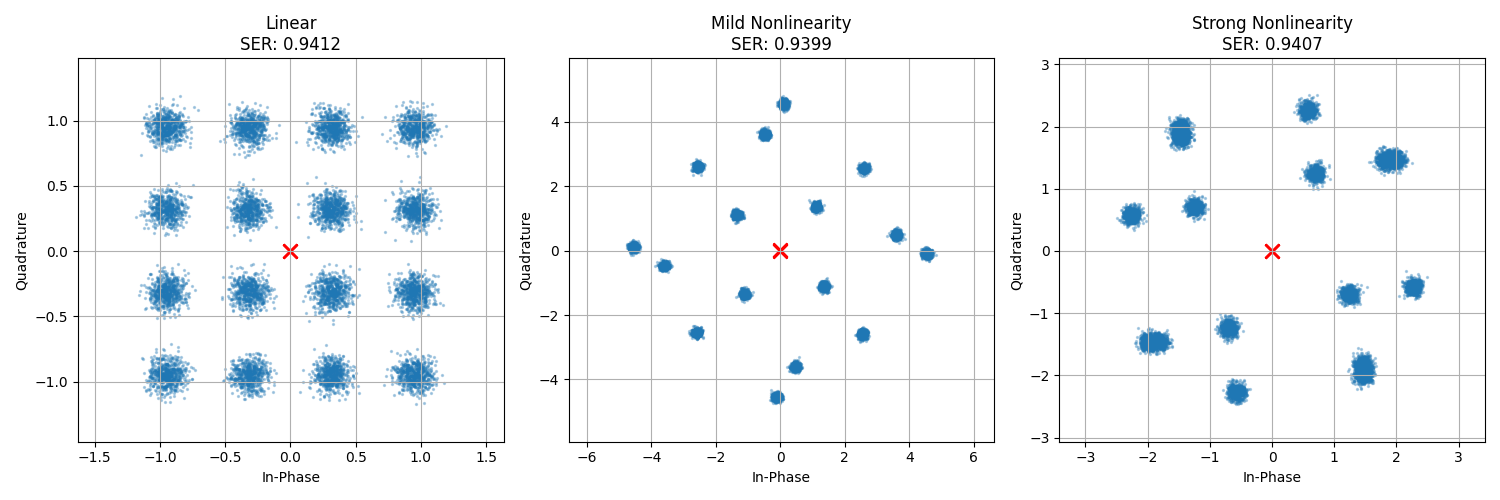
Processed QAM symbols through Linear channel, SER = 0.9412
Processed QAM symbols through Mild Nonlinearity channel, SER = 0.9399
Processed QAM symbols through Strong Nonlinearity channel, SER = 0.9407

Predistortion to Compensate Nonlinearities

Let’s demonstrate how predistortion can mitigate nonlinear effects.

# Define a nonlinearity and its inverse (predistorter)
def cubic_nonlinearity(x, a=0.2):
    """Cubic nonlinearity: y = x + a*x^3"""
    return x + a * x**3


def cubic_predistorter(x, a=0.2):
    """Approximate inverse of cubic nonlinearity (valid for small a)"""
    # Taylor expansion of the inverse function
    return x - a * x**3 + 3 * a**2 * x**5 - 12 * a**3 * x**7


# Create nonlinear channel
nonlinear_param = 0.3
nonlinear_channel = NonlinearChannel(lambda x: cubic_nonlinearity(x, a=nonlinear_param))

# Create test signal - a ramp to clearly show distortion
test_signal = torch.linspace(-1.5, 1.5, 1000).reshape(1, -1)

# Apply different processing chains
with torch.no_grad():
    # Original signal through nonlinear channel
    nonlinear_output = nonlinear_channel(test_signal)

    # Predistorted signal through nonlinear channel
    predistorted = cubic_predistorter(test_signal, a=nonlinear_param)
    compensated_output = nonlinear_channel(predistorted)

# Visualize predistortion effects
plt.figure(figsize=(12, 8))

# Input-output characteristics
plt.subplot(2, 1, 1)
plt.plot(test_signal.numpy().flatten(), test_signal.numpy().flatten(), "k--", label="Linear (Ideal)", linewidth=2)
plt.plot(test_signal.numpy().flatten(), nonlinear_output.numpy().flatten(), "r-", label="Nonlinear", linewidth=2)
plt.plot(test_signal.numpy().flatten(), compensated_output.numpy().flatten(), "g-", label="With Predistortion", linewidth=2)
plt.grid(True)
plt.title("Nonlinearity Compensation through Predistortion")
plt.xlabel("Input Amplitude")
plt.ylabel("Output Amplitude")
plt.legend()

# Plot the predistorter transfer function
plt.subplot(2, 1, 2)
plt.plot(test_signal.numpy().flatten(), test_signal.numpy().flatten(), "k--", label="Linear (Reference)", linewidth=2)
plt.plot(test_signal.numpy().flatten(), predistorted.numpy().flatten(), "b-", label="Predistorter Function", linewidth=2)
plt.grid(True)
plt.title("Predistorter Transfer Function")
plt.xlabel("Input Amplitude")
plt.ylabel("Predistorted Amplitude")
plt.legend()

plt.tight_layout()
plt.show()

Conclusion

This example demonstrates several key aspects of nonlinear channels in communication systems:

• Nonlinearities introduce harmonic distortion in single-tone signals and intermodulation distortion in multi-tone signals

• Different types of nonlinearities (soft clipping, hard clipping, polynomial) produce characteristic spectral effects

• The Saleh model provides a useful characterization of nonlinear power amplifiers through its AM/AM and AM/PM characteristics

• Nonlinear distortion can severely impact digital modulation schemes by warping constellation points, leading to increased symbol error rates

• Predistortion techniques can effectively mitigate nonlinear distortion by applying the inverse nonlinear function before the channel

The NonlinearChannel in Kaira offers a flexible way to model these effects with custom nonlinear functions, supporting both real and complex-valued signals.