Note
Go to the end to download the full example code. or to run this example in your browser via Binder
Rician Fading vs Rayleigh Fading Channels
This example demonstrates the difference between Rician and Rayleigh fading channels in Kaira. While both model multipath propagation in wireless communications, Rician fading includes a dominant line-of-sight component, making it suitable for modeling wireless channels where there is a direct path between transmitter and receiver.
We’ll visualize the effect of different K-factors in Rician fading and compare with Rayleigh fading.
Imports and Setup
import matplotlib.pyplot as plt
import numpy as np
import seaborn as sns
import torch

from kaira.channels import RayleighFadingChannel, RicianFadingChannel
from kaira.metrics.signal import BitErrorRate, SymbolErrorRate
from kaira.modulations import QPSKDemodulator, QPSKModulator

# Set random seed for reproducibility
torch.manual_seed(42)
np.random.seed(42)
Generate QPSK Signal
Let’s create QPSK modulated symbols to transmit through our channels
# Create a QPSK modulator and demodulator
qpsk_modulator = QPSKModulator()
qpsk_demodulator = QPSKDemodulator()

# Generate random bits for transmission
n_symbols = 10000
n_bits = n_symbols * 2  # QPSK uses 2 bits per symbol
random_bits = torch.randint(0, 2, (1, n_bits)).float()

# Modulate bits to QPSK symbols
with torch.no_grad():
    qpsk_symbols = qpsk_modulator(random_bits)
Configure Fading Channels
We’ll create multiple channels with different parameters
# Fixed coherence time for all channels
coherence_time = 50

# Create channels
channels = [
    ("Rayleigh Fading", RayleighFadingChannel(coherence_time=coherence_time, snr_db=15)),
    ("Rician (K=1)", RicianFadingChannel(k_factor=1, coherence_time=coherence_time, snr_db=15)),
    ("Rician (K=5)", RicianFadingChannel(k_factor=5, coherence_time=coherence_time, snr_db=15)),
    ("Rician (K=10)", RicianFadingChannel(k_factor=10, coherence_time=coherence_time, snr_db=15)),
]
Transmit Signals Through Channels
Process the QPSK symbols through each channel
# Set up metrics
ser_metric = SymbolErrorRate()
ber_metric = BitErrorRate()

# Process signals and collect results
channel_outputs: list[tuple[str, torch.Tensor]] = []
fading_coefficients: list[tuple[str, torch.Tensor]] = []
ser_results: list[tuple[str, float]] = []
ber_results: list[tuple[str, float]] = []

for name, channel in channels:
    # Get index of symbols from original bits for later decoding
    with torch.no_grad():
        # Transform input to complex and reshape if needed
        input_complex = qpsk_symbols.view(1, -1)

        # Pass through channel
        output = channel(input_complex)

        # Save outputs for visualization
        channel_outputs.append((name, output))

        # Decode output to make hard decisions
        output_scaled = output / torch.mean(torch.abs(output))
        decoded_bits = qpsk_demodulator(output_scaled)

        # Calculate error metrics
        ser = ser_metric(decoded_bits.view(-1, 2), random_bits.view(-1, 2))
        ber = ber_metric(decoded_bits, random_bits)

        ser_results.append((name, ser.item()))
        ber_results.append((name, ber.item()))

        print(f"{name}: SER = {ser.item():.4f}, BER = {ber.item():.4f}")
Rayleigh Fading: SER = 0.7042, BER = 0.4798
Rician (K=1): SER = 0.3405, BER = 0.1828
Rician (K=5): SER = 0.0450, BER = 0.0249
Rician (K=10): SER = 0.0037, BER = 0.0019
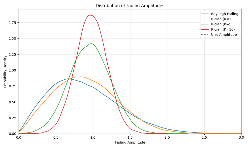
Visualize Fading Channel Amplitude Distributions
Let’s generate and plot the distribution of fading amplitudes for each channel type
plt.figure(figsize=(10, 6))

# Generate samples for each channel type
n_samples = 100000
coherence_time = 1  # Generate independent samples

fading_amplitudes = []
for name, channel in channels:
    # Create a complex input of ones
    x = torch.ones((1, n_samples), dtype=torch.complex64)

    # Turn off noise to isolate fading effect (we'll manually set SNR to a high value)
    if "Rayleigh" in name:
        channel_no_noise = RayleighFadingChannel(coherence_time=coherence_time, snr_db=100)
    else:
        k = float(name.split("K=")[1].split(")")[0]) if "K=" in name else 1
        channel_no_noise = RicianFadingChannel(k_factor=k, coherence_time=coherence_time, snr_db=100)

    # Pass through channel to get fading coefficients
    y = channel_no_noise(x)

    # Calculate amplitude
    amplitudes = torch.abs(y).cpu().numpy().flatten()

    # Save for plotting
    fading_amplitudes.append((name, amplitudes))

# Plot distributions
for name, amplitudes in fading_amplitudes:
    sns.kdeplot(amplitudes, label=name)

# Add vertical line at amplitude=1 for reference
plt.axvline(x=1.0, color="black", linestyle="--", alpha=0.5, label="Unit Amplitude")

plt.xlabel("Fading Amplitude")
plt.ylabel("Probability Density")
plt.title("Distribution of Fading Amplitudes")
plt.legend()
plt.grid(True, alpha=0.3)
plt.xlim(0, 3)
plt.tight_layout()
Visualize Channel Outputs in Constellation Diagram
Let’s see how the different fading channels affect our QPSK signal
fig, axes = plt.subplots(2, 2, figsize=(12, 10))
axes = axes.flatten()

# Get QPSK constellation points for reference
constellation_points = qpsk_modulator.constellation

# Plot each channel's output
for i, (name, output) in enumerate(channel_outputs):
    ax = axes[i]

    # Take a subset for clearer visualization
    subset_size = 1000
    output_subset = output[0, :subset_size].cpu().numpy()

    # Scatter plot
    ax.scatter(output_subset.real, output_subset.imag, s=10, alpha=0.5)

    # Plot original constellation points
    for point in constellation_points:
        ax.plot(point.real, point.imag, "rx", markersize=10)

    # Add circle at unit radius for reference
    circle = plt.Circle((0, 0), 1, fill=False, linestyle="--", color="gray")
    ax.add_patch(circle)

    ax.set_title(f"{name} Channel Output")
    ax.set_xlabel("In-phase")
    ax.set_ylabel("Quadrature")
    ax.grid(True, alpha=0.3)
    ax.set_xlim(-2, 2)
    ax.set_ylim(-2, 2)
    ax.set_aspect("equal")

plt.tight_layout()

Compare Error Rates Across SNR Values
Now let’s see how each channel performs across different SNR levels
snr_range_db = list(range(0, 31, 2))
ser_vs_snr: dict[str, list[float]] = {name: [] for name, _ in channels}
ber_vs_snr: dict[str, list[float]] = {name: [] for name, _ in channels}

for snr_db in snr_range_db:
    for name, channel_type in channels:
        # Recreate channel with the current SNR
        if "Rayleigh" in name:
            channel = RayleighFadingChannel(coherence_time=coherence_time, snr_db=snr_db)
        else:
            k = float(name.split("K=")[1].split(")")[0]) if "K=" in name else 1
            channel = RicianFadingChannel(k_factor=k, coherence_time=coherence_time, snr_db=snr_db)

        # Pass through channel
        with torch.no_grad():
            input_complex = qpsk_symbols.view(1, -1)
            output = channel(input_complex)

            # Decode output
            output_scaled = output / torch.mean(torch.abs(output))
            decoded_bits = qpsk_demodulator(output_scaled)

            # Calculate error metrics
            ser = ser_metric(decoded_bits.view(-1, 2), random_bits.view(-1, 2))
            ber = ber_metric(decoded_bits, random_bits)

            ser_vs_snr[name].append(ser.item())
            ber_vs_snr[name].append(ber.item())
Plot SER vs SNR
plt.figure(figsize=(10, 6))
for name in ser_vs_snr:
    plt.semilogy(snr_range_db, ser_vs_snr[name], "o-", linewidth=2, label=name)

plt.grid(True, which="both", linestyle="--", alpha=0.6)
plt.xlabel("SNR (dB)")
plt.ylabel("Symbol Error Rate")
plt.title("Symbol Error Rate vs SNR for Different Fading Channels")
plt.legend()
plt.tight_layout()

Plot BER vs SNR
plt.figure(figsize=(10, 6))
for name in ber_vs_snr:
    plt.semilogy(snr_range_db, ber_vs_snr[name], "o-", linewidth=2, label=name)

plt.grid(True, which="both", linestyle="--", alpha=0.6)
plt.xlabel("SNR (dB)")
plt.ylabel("Bit Error Rate")
plt.title("Bit Error Rate vs SNR for Different Fading Channels")
plt.legend()
plt.tight_layout()

Conclusion
This example demonstrates the key differences between Rayleigh and Rician fading:
Rayleigh fading models environments with no direct line-of-sight (NLOS) path, resulting in all signal components arriving from indirect reflections. The amplitude distribution has its peak at values below 1 and has higher probability of very deep fades.
Rician fading models environments with a dominant direct line-of-sight (LOS) component plus multiple reflected paths. The K-factor controls the ratio of power in the direct path to the power in the reflected paths:
With higher K-factors, the amplitude distribution shifts right and becomes more Gaussian-like
Higher K-factors result in better performance (lower error rates)
As K approaches zero, Rician fading becomes equivalent to Rayleigh fading
As K approaches infinity, Rician fading approaches an AWGN channel (no fading)
These channel models are critical for accurately simulating wireless systems in different environments, such as:
Rayleigh: Urban areas, indoor environments with many obstacles
Rician (low K): Suburban areas with partial line-of-sight
Rician (high K): Rural areas or satellite communications with strong direct path
Kaira provides implementations of both channel types with configurable parameters to support realistic wireless communication simulations.
Total running time of the script: (0 minutes 2.653 seconds)
