Adversarial Losses for GANs

This example demonstrates the various adversarial losses available in kaira for training Generative Adversarial Networks (GANs).

We’ll cover: - Vanilla GAN Loss - Wasserstein GAN Loss (WGAN) - Least Squares GAN Loss (LSGAN) - Hinge Loss

from typing import Dict, List

import matplotlib.pyplot as plt

First, let’s import the necessary modules

import torch

from kaira.losses import LossRegistry

Let’s create some sample data to simulate discriminator outputs

batch_size = 128
real_logits = torch.randn(batch_size, 1) + 2.0  # Center around 2 for real samples
fake_logits = torch.randn(batch_size, 1) - 2.0  # Center around -2 for fake samples

Now let’s compare how different GAN losses behave

# Vanilla GAN Loss
vanilla_gan = LossRegistry.create("vanillaganloss")  # Changed from 'vanillagan' to 'vanillaganloss'
vanilla_d_loss = vanilla_gan.forward_discriminator(real_logits, fake_logits)
vanilla_g_loss = vanilla_gan.forward_generator(fake_logits)
print(f"Vanilla GAN - D Loss: {vanilla_d_loss:.4f}, G Loss: {vanilla_g_loss:.4f}")

# Wasserstein GAN Loss
wgan = LossRegistry.create("wassersteinganloss")
wgan_d_loss = wgan.forward_discriminator(real_logits, fake_logits)
wgan_g_loss = wgan.forward_generator(fake_logits)
print(f"WGAN - D Loss: {wgan_d_loss:.4f}, G Loss: {wgan_g_loss:.4f}")

# LSGAN Loss
lsgan = LossRegistry.create("lsganloss")
lsgan_d_loss = lsgan.forward_discriminator(real_logits, fake_logits)
lsgan_g_loss = lsgan.forward_generator(fake_logits)
print(f"LSGAN - D Loss: {lsgan_d_loss:.4f}, G Loss: {lsgan_g_loss:.4f}")

# Hinge Loss
hinge = LossRegistry.create("hingeloss")
hinge_d_loss = hinge.forward_discriminator(real_logits, fake_logits)
hinge_g_loss = hinge.forward_generator(fake_logits)
print(f"Hinge - D Loss: {hinge_d_loss:.4f}, G Loss: {hinge_g_loss:.4f}")

Vanilla GAN - D Loss: 0.3493, G Loss: 2.1376
WGAN - D Loss: -4.0124, G Loss: 1.9500
LSGAN - D Loss: 3.3296, G Loss: 9.6696
Hinge - D Loss: 0.1453, G Loss: 1.9500

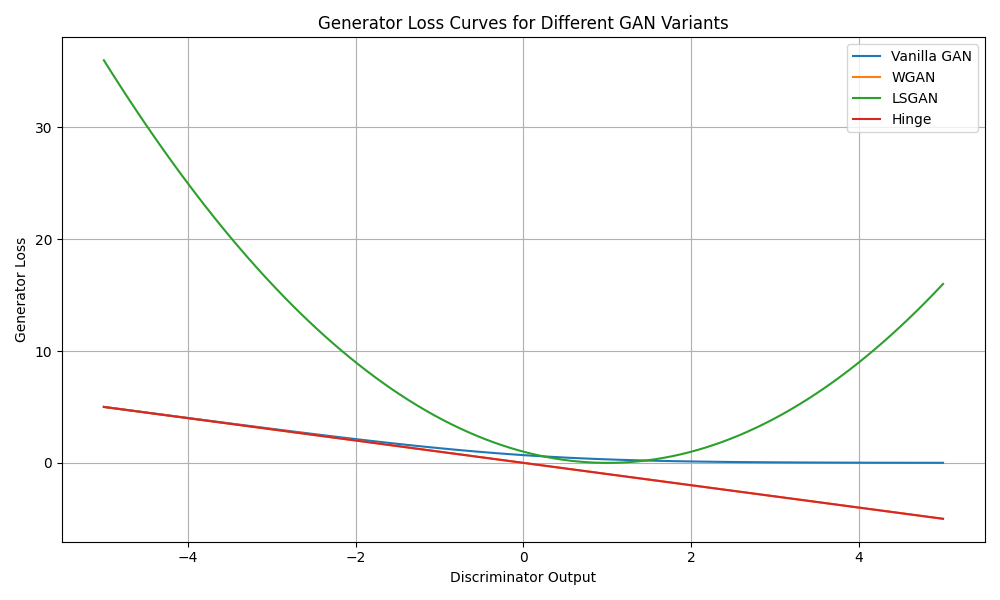
Let’s visualize how these losses respond to different discriminator outputs

def compute_losses(d_output):
    """Compute different GAN losses for a given discriminator output."""
    # Assume we're computing generator loss
    losses = {"Vanilla GAN": vanilla_gan.forward_generator(d_output), "WGAN": wgan.forward_generator(d_output), "LSGAN": lsgan.forward_generator(d_output), "Hinge": hinge.forward_generator(d_output)}
    return {k: v.item() for k, v in losses.items()}


# Generate range of discriminator outputs
d_outputs = torch.linspace(-5, 5, 100).unsqueeze(1)
loss_curves: Dict[str, List[float]] = {name: [] for name in ["Vanilla GAN", "WGAN", "LSGAN", "Hinge"]}

for d_out in d_outputs:
    losses = compute_losses(d_out.unsqueeze(0))
    for name, loss in losses.items():
        loss_curves[name].append(loss)

Plot the generator loss curves

plt.figure(figsize=(10, 6))
for name, losses in loss_curves.items():
    plt.plot(d_outputs.squeeze().numpy(), losses, label=name)

plt.xlabel("Discriminator Output")
plt.ylabel("Generator Loss")
plt.title("Generator Loss Curves for Different GAN Variants")
plt.legend()
plt.grid(True)
plt.tight_layout()
plt.show()

Let’s also visualize how the discriminator losses behave

def compute_d_losses(real_out, fake_out):
    """Compute discriminator losses for given real and fake outputs."""
    real_batch = real_out.expand(batch_size, 1)
    fake_batch = fake_out.expand(batch_size, 1)

    losses = {"Vanilla GAN": vanilla_gan.forward_discriminator(real_batch, fake_batch), "WGAN": wgan.forward_discriminator(real_batch, fake_batch), "LSGAN": lsgan.forward_discriminator(real_batch, fake_batch), "Hinge": hinge.forward_discriminator(real_batch, fake_batch)}
    return {k: v.item() for k, v in losses.items()}


# Generate combinations of real and fake outputs
real_range = torch.linspace(-2, 4, 20)
fake_range = torch.linspace(-4, 2, 20)
X, Y = torch.meshgrid(real_range, fake_range, indexing="ij")
Z = {name: torch.zeros_like(X) for name in ["Vanilla GAN", "WGAN", "LSGAN", "Hinge"]}

for i in range(len(real_range)):
    for j in range(len(fake_range)):
        losses = compute_d_losses(real_range[i].unsqueeze(0), fake_range[j].unsqueeze(0))
        for name, loss in losses.items():
            Z[name][i, j] = loss

Plot discriminator loss surfaces

fig = plt.figure(figsize=(15, 10))
for idx, (name, loss_surface) in enumerate(Z.items(), 1):
    ax = fig.add_subplot(2, 2, idx, projection="3d")
    surf = ax.plot_surface(X.numpy(), Y.numpy(), loss_surface.numpy(), cmap="viridis")  # type: ignore[attr-defined]
    ax.set_xlabel("Real Output")
    ax.set_ylabel("Fake Output")
    ax.set_zlabel("Loss")  # type: ignore[attr-defined]
    ax.set_title(f"{name} Discriminator Loss")
    fig.colorbar(surf, ax=ax, shrink=0.5, aspect=5)

plt.tight_layout()
plt.show()

This example illustrates the different behaviors of various GAN loss functions: - Vanilla GAN uses the original binary cross-entropy loss - WGAN directly optimizes the Wasserstein distance - LSGAN uses least squares loss for more stable training - Hinge loss provides an alternative formulation with margin

The visualization shows how these losses respond differently to discriminator outputs, which can affect training dynamics and stability. WGAN and LSGAN typically provide more stable training compared to the original GAN loss.