Image Losses for Image Quality Assessment

This example demonstrates the various image losses available in kaira for assessing image quality and training image-based models.

We’ll cover: - MSE Loss (Mean Squared Error) - LPIPS Loss (Learned Perceptual Image Patch Similarity) - SSIM Loss (Structural Similarity Index) - Combined Loss (Multiple losses with weights)

from typing import Dict, List

import matplotlib.pyplot as plt
import numpy as np

First, let’s import the necessary modules

import torch
import torch.nn as nn

from kaira.losses import LossRegistry

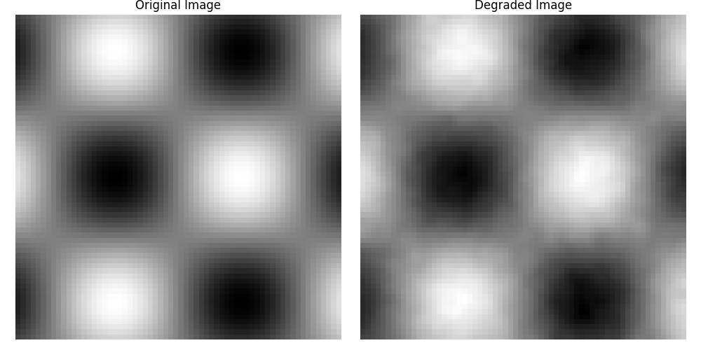
Create sample data - we’ll simulate an original image and a degraded version For this example, we’ll create simple synthetic images

def create_sample_images(size=64):
    """Create synthetic image pairs for demonstrating image quality losses.

    Generates a pattern image using sinusoidal functions and a degraded version
    of the same image with added noise and Gaussian blur.

    Args:
        size (int): The width and height of the square images to generate.
                   Defaults to 64.

    Returns:
        tuple: A pair of torch tensors (original, degraded) where:
            - original: Clean pattern image of shape (1, 1, size, size)
            - degraded: Noisy/blurred version of shape (1, 1, size, size)
            Both tensors are normalized to [0, 1] range.
    """
    # Create an original image with a pattern
    x = np.linspace(-4, 4, size)
    y = np.linspace(-4, 4, size)
    xx, yy = np.meshgrid(x, y)
    original = np.sin(xx) * np.cos(yy)

    # Create a degraded version with noise and blur
    degraded = original + np.random.normal(0, 0.1, original.shape)
    from scipy.ndimage import gaussian_filter

    degraded = gaussian_filter(degraded, sigma=1.0)

    # Normalize to [0, 1] range
    original = (original - original.min()) / (original.max() - original.min())
    degraded = (degraded - degraded.min()) / (degraded.max() - degraded.min())

    # Convert to torch tensors with batch and channel dimensions
    original = torch.from_numpy(original).float().unsqueeze(0).unsqueeze(0)
    degraded = torch.from_numpy(degraded).float().unsqueeze(0).unsqueeze(0)

    return original, degraded


# Create sample images
original, degraded = create_sample_images()

# Convert to 3 channels for LPIPS
original_3ch = original.repeat(1, 3, 1, 1)
degraded_3ch = degraded.repeat(1, 3, 1, 1)

# Normalize to [-1, 1] for LPIPS
original_3ch_norm = (original_3ch * 2) - 1
degraded_3ch_norm = (degraded_3ch * 2) - 1


# Helper function to ensure images are properly normalized to [-1, 1] range
def ensure_normalized(tensor):
    """Normalize tensor to [-1, 1] range regardless of current range."""
    tensor_min = tensor.min()
    tensor_max = tensor.max()
    return 2 * (tensor - tensor_min) / (tensor_max - tensor_min) - 1

Let’s visualize our sample images

plt.figure(figsize=(10, 5))
plt.subplot(121)
plt.imshow(original.squeeze(), cmap="gray")
plt.title("Original Image")
plt.axis("off")
plt.subplot(122)
plt.imshow(degraded.squeeze(), cmap="gray")
plt.title("Degraded Image")
plt.axis("off")
plt.tight_layout()
plt.show()

Now let’s compute different losses between the original and degraded images

# MSE Loss
mse_loss = LossRegistry.create("mseloss")
mse_value = mse_loss(degraded, original).item()
print(f"MSE Loss: {mse_value:.4f}")

# SSIM Loss
ssim_loss = LossRegistry.create("ssimloss")
ssim_value = ssim_loss(degraded, original).item()
print(f"SSIM Loss: {ssim_value:.4f}")

# LPIPS Loss
lpips_loss = LossRegistry.create("lpipsloss")
# Now compute LPIPS with normalized inputs
lpips_value = lpips_loss(degraded_3ch_norm, original_3ch_norm).item()
print(f"LPIPS Loss: {lpips_value:.4f}")

MSE Loss: 0.0003
SSIM Loss: 0.0263
LPIPS Loss: 0.0516

Let’s create a combined loss with different weights

combined_loss = LossRegistry.create("combinedloss", losses=[mse_loss, ssim_loss], weights=[0.7, 0.3])
combined_value = combined_loss(degraded, original).item()
print(f"Combined Loss (0.7*MSE + 0.3*SSIM): {combined_value:.4f}")

Combined Loss (0.7*MSE + 0.3*SSIM): 0.0081

Let’s see how different losses respond to various types of image degradation

def apply_degradation(image, degradation_type, param):
    """Apply different types of degradation to an image."""
    if degradation_type == "gaussian_noise":
        return image + torch.randn_like(image) * param
    elif degradation_type == "blur":
        kernel_size = int(param)
        if kernel_size % 2 == 0:
            kernel_size += 1
        return nn.functional.avg_pool2d(image, kernel_size=kernel_size, stride=1, padding=kernel_size // 2)
    return image


# Create functions for different types of degradation
def add_gaussian_noise(image, std=0.1):
    """Add Gaussian noise to an image tensor."""
    return image + torch.randn_like(image) * std


# Create a range of degradation parameters
noise_levels = np.linspace(0, 0.5, 10)
blur_sizes = np.arange(1, 20, 2)

# Store results
noise_results: Dict[str, List[float]] = {"mse": [], "ssim": [], "lpips": []}
blur_results: Dict[str, List[float]] = {"mse": [], "ssim": [], "lpips": []}

# Compute losses for different noise levels
for noise in noise_levels:
    noisy = apply_degradation(original, "gaussian_noise", noise)
    noisy_3ch = noisy.repeat(1, 3, 1, 1)

    # Normalize inputs to [-1, 1] for LPIPS
    noisy_3ch_norm = ensure_normalized(noisy_3ch)
    original_3ch_norm = ensure_normalized(original_3ch)

    noise_results["mse"].append(mse_loss(noisy, original).item())
    noise_results["ssim"].append(ssim_loss(noisy, original).item())
    noise_results["lpips"].append(lpips_loss(noisy_3ch_norm, original_3ch_norm).item())

# Compute losses for different blur levels
for blur in blur_sizes:
    blurred = apply_degradation(original, "blur", blur)
    blurred_3ch = blurred.repeat(1, 3, 1, 1)

    # Normalize inputs to [-1, 1] for LPIPS
    blurred_3ch_norm = ensure_normalized(blurred_3ch)
    original_3ch_norm = ensure_normalized(original_3ch)

    blur_results["mse"].append(mse_loss(blurred, original).item())
    blur_results["ssim"].append(ssim_loss(blurred, original).item())
    blur_results["lpips"].append(lpips_loss(blurred_3ch_norm, original_3ch_norm).item())

Plot the results

plt.figure(figsize=(12, 5))

plt.subplot(121)
plt.plot(noise_levels, noise_results["mse"], label="MSE Loss")
plt.plot(noise_levels, noise_results["ssim"], label="SSIM Loss")
plt.plot(noise_levels, noise_results["lpips"], label="LPIPS Loss")
plt.xlabel("Noise Level (σ)")
plt.ylabel("Loss Value")
plt.title("Loss Response to Gaussian Noise")
plt.legend()

plt.subplot(122)
plt.plot(blur_sizes, blur_results["mse"], label="MSE Loss")
plt.plot(blur_sizes, blur_results["ssim"], label="SSIM Loss")
plt.plot(blur_sizes, blur_results["lpips"], label="LPIPS Loss")
plt.xlabel("Blur Kernel Size")
plt.ylabel("Loss Value")
plt.title("Loss Response to Blur")
plt.legend()

plt.tight_layout()
plt.show()

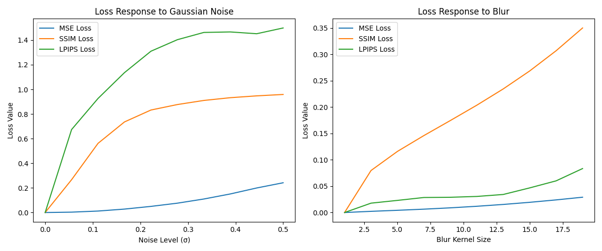
This example shows how different losses respond differently to various types of image degradation. MSE is simple but doesn’t always correlate well with human perception. SSIM better captures structural information, while LPIPS aims to match human perceptual judgments. Using a combination of losses often leads to better results in practice.