Text Losses for NLP Tasks

This example demonstrates the various text-based losses available in kaira for training natural language processing models.

We’ll cover: - Cross Entropy Loss - Label Smoothing Loss - Word2Vec Loss - Cosine Similarity Loss

import matplotlib.pyplot as plt
import numpy as np

First, let’s import the necessary modules

import torch
import torch.nn as nn

from kaira.losses import LossRegistry

Let’s create some sample data for text classification

def create_sample_classification_data(n_samples=100, n_classes=5):
    """Create synthetic data for text classification tasks.

    Args:
        n_samples (int): Number of samples to generate.
        n_classes (int): Number of classification classes.

    Returns:
        tuple: (logits, labels) where logits are model outputs and labels are true classes.
    """
    # Create logits (raw model outputs)
    logits = torch.randn(n_samples, n_classes)

    # Create true labels
    labels = torch.randint(0, n_classes, (n_samples,))

    return logits, labels


# Create classification samples
logits, labels = create_sample_classification_data()

Now let’s compare standard cross-entropy with label smoothing

# Standard Cross Entropy Loss
ce_loss = LossRegistry.create("crossentropyloss")
ce_value = ce_loss(logits, labels)
print(f"Cross Entropy Loss: {ce_value:.4f}")

# Label Smoothing Loss (with different smoothing values)
smoothing_values = [0.0, 0.1, 0.2, 0.3]
for smoothing in smoothing_values:
    ls_loss = LossRegistry.create("labelsmoothingloss", smoothing=smoothing, classes=5)
    ls_value = ls_loss(logits, labels)
    print(f"Label Smoothing Loss (α={smoothing}): {ls_value:.4f}")

Cross Entropy Loss: 2.0786
Label Smoothing Loss (α=0.0): 2.0786
Label Smoothing Loss (α=0.1): 2.0699
Label Smoothing Loss (α=0.2): 2.0613
Label Smoothing Loss (α=0.3): 2.0526

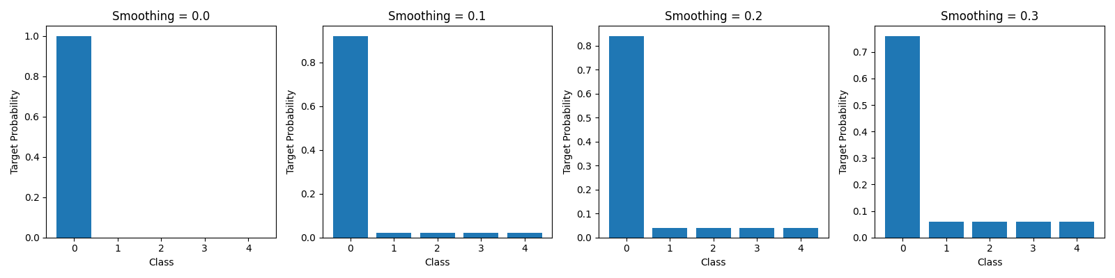
Let’s visualize how label smoothing affects the target distribution

def plot_label_distributions(smoothing_values, n_classes=5):
    """Visualize how label smoothing affects the target distribution.

    Args:
        smoothing_values (list): List of label smoothing values to visualize.
        n_classes (int): Number of classes in the distribution.
    """
    fig, axes = plt.subplots(1, len(smoothing_values), figsize=(4 * len(smoothing_values), 4))

    for i, smoothing in enumerate(smoothing_values):
        # Create target distribution
        target_dist = torch.zeros(n_classes)
        target_dist[0] = 1.0  # true class

        if smoothing > 0:
            target_dist = target_dist * (1 - smoothing) + smoothing / n_classes

        axes[i].bar(range(n_classes), target_dist)
        axes[i].set_title(f"Smoothing = {smoothing}")
        axes[i].set_xlabel("Class")
        axes[i].set_ylabel("Target Probability")

    plt.tight_layout()
    plt.show()


plot_label_distributions(smoothing_values)

Now let’s examine Word2Vec loss for word embeddings

def create_sample_word_embeddings(vocab_size=1000, embed_dim=100):
    """Create sample word embeddings for demonstration.

    Args:
        vocab_size (int): Size of the vocabulary.
        embed_dim (int): Dimension of the embeddings.

    Returns:
        tuple: (embeddings, center_words, context_words) for Word2Vec training.
    """
    # Create sample word embeddings
    embeddings = torch.randn(vocab_size, embed_dim)
    embeddings = nn.functional.normalize(embeddings, p=2, dim=1)

    # Create sample word indices
    center_words = torch.randint(0, vocab_size, (50,))
    context_words = torch.randint(0, vocab_size, (50,))

    return embeddings, center_words, context_words


# Create word embedding samples
embeddings, center_words, context_words = create_sample_word_embeddings()

# Word2Vec Loss
w2v_loss = LossRegistry.create("word2vecloss", embedding_dim=100, vocab_size=1000, n_negatives=5)
w2v_value = w2v_loss(center_words, context_words)
print(f"Word2Vec Loss: {w2v_value:.4f}")

Word2Vec Loss: 4.1589

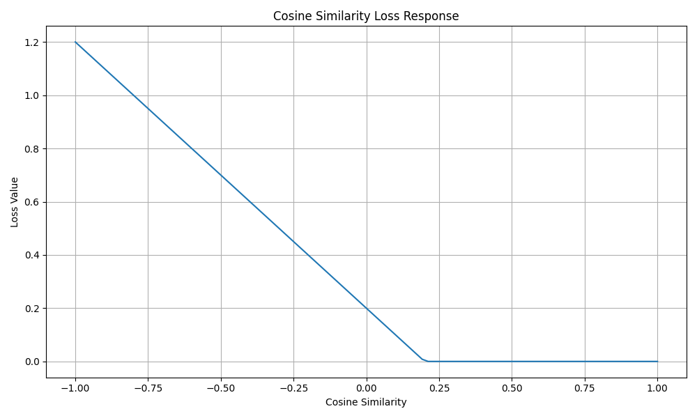
Let’s visualize how the cosine similarity loss behaves for word embeddings

def compute_cosine_losses(similarities):
    """Compute cosine similarity losses for given similarity values.

    Args:
        similarities (numpy.ndarray): Array of cosine similarity values.

    Returns:
        list: Computed loss values for each similarity value.
    """
    # Create pairs of vectors with specified cosine similarities
    v1 = torch.tensor([[1.0, 0.0]])
    losses = []

    for sim in similarities:
        v2 = torch.tensor([[sim, np.sqrt(1 - sim**2)]])
        v1_batch = v1.expand(10, 2)
        v2_batch = v2.expand(10, 2)

        cos_loss = LossRegistry.create("cosinesimilarityloss", margin=0.2)
        loss = cos_loss(v1_batch, v2_batch).item()
        losses.append(loss)

    return losses


# Generate range of similarity values
similarities = np.linspace(-1, 1, 100)
cosine_losses = compute_cosine_losses(similarities)

plt.figure(figsize=(10, 6))
plt.plot(similarities, cosine_losses)
plt.xlabel("Cosine Similarity")
plt.ylabel("Loss Value")
plt.title("Cosine Similarity Loss Response")
plt.grid(True)
plt.tight_layout()
plt.show()

Let’s examine how different losses handle prediction confidence

def plot_confidence_impact():
    """Visualize how different losses respond to prediction confidence.

    Compares Cross Entropy and Label Smoothing losses across confidence levels.
    """
    # Create a range of prediction confidences
    confidences = np.linspace(0.01, 0.99, 100)
    losses = {"Cross Entropy": [], "Label Smoothing (α=0.1)": [], "Label Smoothing (α=0.2)": []}

    # Compute losses for different confidence levels
    for conf in confidences:
        # Create logits that would produce these confidences
        logit = np.log(conf / (1 - conf))
        pred = torch.tensor([[logit, -logit]])
        label = torch.tensor([0])

        # Compute different losses
        losses["Cross Entropy"].append(ce_loss(pred, label).item())
        losses["Label Smoothing (α=0.1)"].append(LossRegistry.create("labelsmoothingloss", smoothing=0.1, classes=2)(pred, label).item())
        losses["Label Smoothing (α=0.2)"].append(LossRegistry.create("labelsmoothingloss", smoothing=0.2, classes=2)(pred, label).item())

    # Plot results
    plt.figure(figsize=(10, 6))
    for name, loss_values in losses.items():
        plt.plot(confidences, loss_values, label=name)

    plt.xlabel("Prediction Confidence")
    plt.ylabel("Loss Value")
    plt.title("Loss Response to Prediction Confidence")
    plt.legend()
    plt.grid(True)
    plt.tight_layout()
    plt.show()


plot_confidence_impact()

This example demonstrates various losses used in NLP tasks:

• Cross Entropy Loss is the standard loss for classification tasks, providing direct probability interpretation.

• Label Smoothing Loss prevents overconfident predictions by distributing some probability mass to non-target classes.

• Word2Vec Loss is used for learning word embeddings through context prediction, capturing semantic relationships between words.

• Cosine Similarity Loss is useful for tasks that compare text embeddings, like sentence similarity or document retrieval.

The visualizations show how label smoothing affects target distributions and how different losses respond to prediction confidence.