Composite Metrics

This example demonstrates how to use and create composite metrics in the Kaira library. Composite metrics allow you to combine multiple metrics into a single entity, which is useful for multi-objective evaluation of communication systems.

import matplotlib.pyplot as plt

Imports and Setup

import numpy as np
import torch

from kaira.metrics import BaseMetric
from kaira.metrics.image import PSNR, SSIM
from kaira.metrics.signal import BER, SNR

# Set random seed for reproducibility
torch.manual_seed(42)
np.random.seed(42)

1. Creating a Composite Metric

We’ll first create a composite metric that combines BER and SNR

# Initialize individual metrics
ber_metric = BER()
snr_metric = SNR()


# Create a wrapper metric that handles both BER and SNR inputs
class BERSNRMetric(BaseMetric):
    """Combined metric for evaluating both Bit Error Rate (BER) and Signal-to-Noise Ratio (SNR).

    Args:
        ber_metric (BER): Instance of BER metric
        snr_metric (SNR): Instance of SNR metric
    """

    def __init__(self, ber_metric, snr_metric):
        super().__init__()
        self.ber = ber_metric
        self.snr = snr_metric

    def forward(self, x, y=None):
        """Calculate both BER and SNR metrics.

        Args:
            x (tuple): Tuple containing (received_bits, original_bits, received_signal, original_signal)
            y (None): Not used, maintained for compatibility

        Returns:
            dict: Dictionary containing 'BER' and 'SNR' values
        """
        # For this metric, x is a tuple containing all needed inputs
        received_bits, bits, received_signal, signal = x
        ber_value = self.ber(received_bits, bits)
        snr_value = self.snr(received_signal, signal)
        return {"BER": ber_value, "SNR": snr_value}


# Create the wrapped metric
wrapped_metric = BERSNRMetric(ber_metric, snr_metric)

# Generate some test data
n_bits = 1000
bits = torch.randint(0, 2, (1, n_bits))
# Introduce some errors (5% error rate)
error_probability = 0.05
errors = torch.rand(1, n_bits) < error_probability
received_bits = torch.logical_xor(bits, errors).int()

# For SNR calculation, we need a signal
signal = (2 * bits - 1.0).float()  # Convert 0/1 bits to -1.0/+1.0 signal
noise = 0.2 * torch.randn_like(signal)
received_signal = signal + noise

# Calculate metrics directly
inputs = (received_bits, bits, received_signal, signal)
result = wrapped_metric(inputs)
print("Metrics Results:")
print(f"BER: {result['BER'].item():.5f}")
print(f"SNR: {result['SNR'].item():.2f} dB")

Metrics Results:
BER: 0.04000
SNR: 14.14 dB

2. Weighted Composite Metrics

Creating a weighted composite metric with custom weights

class WeightedBERSNRMetric(BERSNRMetric):
    """Weighted combination of BER and SNR metrics with normalization.

    Args:
        ber_metric (BER): Instance of BER metric
        snr_metric (SNR): Instance of SNR metric
        ber_weight (float): Weight for BER metric (default: 0.7)
        snr_weight (float): Weight for SNR metric (default: 0.3)
    """

    def __init__(self, ber_metric, snr_metric, ber_weight=0.7, snr_weight=0.3):
        super().__init__(ber_metric, snr_metric)
        total_weight = ber_weight + snr_weight
        self.ber_weight = ber_weight / total_weight
        self.snr_weight = snr_weight / total_weight

    def forward(self, x, y=None):
        """Calculate weighted combination of normalized BER and SNR metrics.

        Args:
            x (tuple): Tuple containing (received_bits, original_bits, received_signal, original_signal)
            y (None): Not used, maintained for compatibility

        Returns:
            dict: Dictionary containing raw metrics, normalized metrics, and weighted score
        """
        results = super().forward(x)
        # Normalize SNR (assuming max SNR of 20 dB for demo)
        norm_snr = torch.clamp(results["SNR"] / 20.0, 0, 1)
        # Invert BER since lower is better (assuming max BER of 0.5)
        norm_ber = 1.0 - torch.clamp(results["BER"] / 0.5, 0, 1)

        weighted_result = self.ber_weight * norm_ber + self.snr_weight * norm_snr

        return {"BER": results["BER"], "SNR": results["SNR"], "BER_normalized": norm_ber, "SNR_normalized": norm_snr, "weighted_score": weighted_result}


# Create a weighted metric
weighted_metric = WeightedBERSNRMetric(ber_metric, snr_metric)

# Calculate weighted result
result_weighted = weighted_metric(inputs)
print("\nWeighted Metrics Result:")
print(f"BER: {result_weighted['BER'].item():.5f}")
print(f"SNR: {result_weighted['SNR'].item():.2f} dB")
print(f"Normalized BER: {result_weighted['BER_normalized'].item():.5f}")
print(f"Normalized SNR: {result_weighted['SNR_normalized'].item():.5f}")
print(f"Weighted Score: {result_weighted['weighted_score'].item():.5f}")

Weighted Metrics Result:
BER: 0.04000
SNR: 14.14 dB
Normalized BER: 0.92000
Normalized SNR: 0.70698
Weighted Score: 0.85609

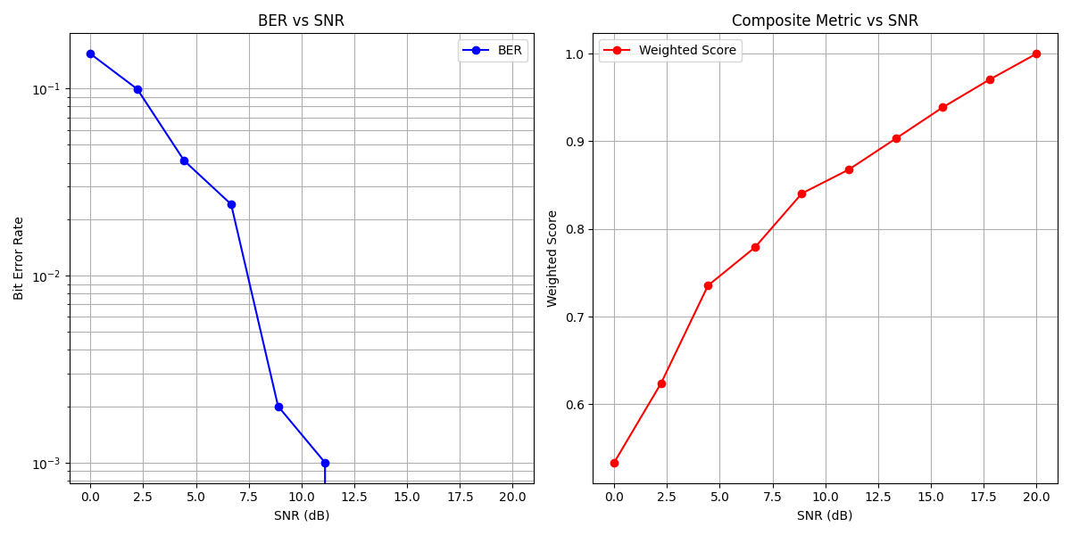
3. Visualizing Metric Trade-offs

Creating a chart to show how different metrics behave

# Generate data with varying SNR
snr_db_range = torch.linspace(0, 20, 10)
ber_values = []
snr_values = []
weighted_scores = []

# Simple model of BER vs SNR for BPSK in AWGN
# BER = 0.5 * erfc(sqrt(SNR))
for snr_db in snr_db_range:
    # Calculate theoretical BER for this SNR
    snr_linear = 10 ** (snr_db.item() / 10)
    ber = 0.5 * torch.erfc(torch.sqrt(torch.tensor(snr_linear)) / torch.sqrt(torch.tensor(2.0)))

    # Create signals for this SNR
    this_signal = torch.ones((1, n_bits)) * 1.0
    noise_power = 1.0 / snr_linear
    this_noise = torch.sqrt(torch.tensor(noise_power)) * torch.randn_like(this_signal)
    this_received = this_signal + this_noise

    # Generate bits with error rate matching the theoretical BER
    this_bits = torch.ones((1, n_bits), dtype=torch.int)
    error_mask = torch.rand(1, n_bits) < ber
    this_received_bits = torch.logical_xor(this_bits, error_mask).int()

    # Calculate metrics
    this_inputs = (this_received_bits, this_bits, this_received, this_signal)
    this_result = weighted_metric(this_inputs)

    # Store results
    ber_values.append(this_result["BER"].item())
    snr_values.append(snr_db.item())
    weighted_scores.append(this_result["weighted_score"].item())

# Plot results
plt.figure(figsize=(12, 6))

# First subplot: BER vs SNR
plt.subplot(1, 2, 1)
plt.semilogy(snr_db_range, ber_values, "bo-", label="BER")
plt.grid(True, which="both")
plt.xlabel("SNR (dB)")
plt.ylabel("Bit Error Rate")
plt.title("BER vs SNR")
plt.legend()

# Second subplot: Weighted score vs SNR
plt.subplot(1, 2, 2)
plt.plot(snr_db_range, weighted_scores, "ro-", label="Weighted Score")
plt.grid(True)
plt.xlabel("SNR (dB)")
plt.ylabel("Weighted Score")
plt.title("Composite Metric vs SNR")
plt.legend()

plt.tight_layout()
plt.show()

4. Creating a Custom Composite Metric for Image Quality

Combining PSNR and SSIM metrics with custom weights

# Generate test images
def create_test_image(size=64):
    """Create a simple test image pattern."""
    x = np.linspace(-4, 4, size)
    y = np.linspace(-4, 4, size)
    xx, yy = np.meshgrid(x, y)
    # Create a pattern with some features
    z = np.sin(xx) * np.cos(yy)
    return torch.FloatTensor(z).unsqueeze(0).unsqueeze(0)


# Create original and noisy images
original_img = create_test_image()
noisy_img = original_img + 0.1 * torch.randn_like(original_img)

# Create PSNR and SSIM metrics
psnr_metric = PSNR(data_range=2.0)  # Range is [-1,1]
ssim_metric = SSIM(data_range=2.0)  # Range is [-1,1]


# Create a custom image quality metric
class ImageQualityMetric(BaseMetric):
    """Combined image quality metric using PSNR and SSIM.

    Args:
        psnr_metric (PSNR): Instance of PSNR metric
        ssim_metric (SSIM): Instance of SSIM metric
        psnr_weight (float): Weight for PSNR metric (default: 0.4)
        ssim_weight (float): Weight for SSIM metric (default: 0.6)
    """

    def __init__(self, psnr_metric, ssim_metric, psnr_weight=0.4, ssim_weight=0.6):
        super().__init__()
        self.psnr = psnr_metric
        self.ssim = ssim_metric
        total_weight = psnr_weight + ssim_weight
        self.psnr_weight = psnr_weight / total_weight
        self.ssim_weight = ssim_weight / total_weight

    def forward(self, x, y):
        """Calculate weighted combination of PSNR and SSIM metrics.

        Args:
            x (torch.Tensor): Input image
            y (torch.Tensor): Reference image

        Returns:
            dict: Dictionary containing PSNR, SSIM, normalized PSNR, and weighted score
        """
        # Calculate individual metrics
        psnr_value = self.psnr(x, y)
        ssim_value = self.ssim(x, y)

        # Normalize PSNR to [0,1] (assuming max PSNR is 50 dB)
        norm_psnr = torch.clamp(psnr_value / 50.0, 0, 1)

        # Combine into a weighted score
        weighted_score = self.psnr_weight * norm_psnr + self.ssim_weight * ssim_value

        return {"PSNR": psnr_value, "SSIM": ssim_value, "PSNR_normalized": norm_psnr, "weighted_score": weighted_score}


# Create image quality metric
img_quality_metric = ImageQualityMetric(psnr_metric, ssim_metric)

# Evaluate image quality
img_result = img_quality_metric(noisy_img, original_img)
print("\nImage Quality Evaluation:")
print(f"PSNR: {img_result['PSNR'].item():.2f} dB")
print(f"SSIM: {img_result['SSIM'].item():.4f}")
print(f"Normalized PSNR: {img_result['PSNR_normalized'].item():.4f}")
print(f"Weighted Score: {img_result['weighted_score'].item():.4f}")

# Visualize the images
plt.figure(figsize=(10, 4))
plt.subplot(1, 2, 1)
plt.imshow(original_img[0, 0].numpy(), cmap="gray")
plt.title("Original Image")
plt.colorbar()

plt.subplot(1, 2, 2)
plt.imshow(noisy_img[0, 0].numpy(), cmap="gray")
plt.title(f'Noisy Image (PSNR: {img_result["PSNR"].item():.1f} dB, SSIM: {img_result["SSIM"].item():.3f})')
plt.colorbar()

plt.tight_layout()
plt.show()

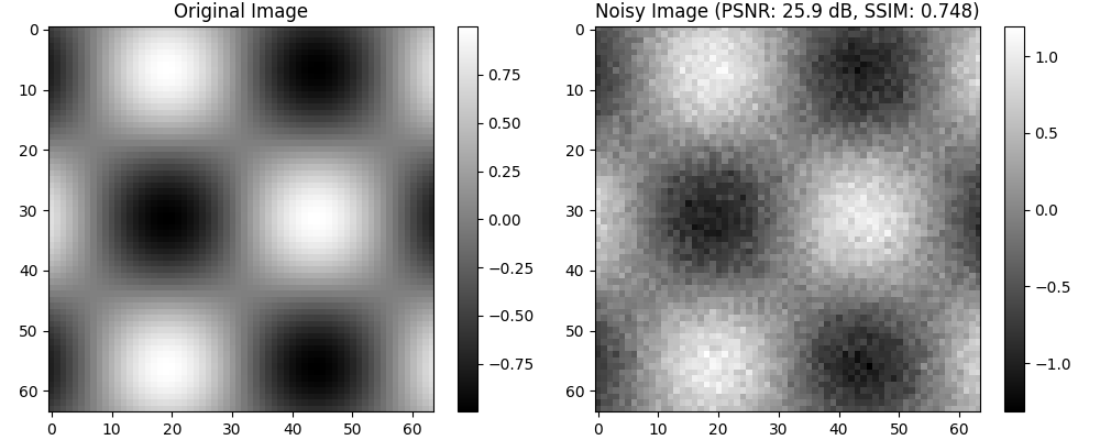
Image Quality Evaluation:
PSNR: 25.93 dB
SSIM: 0.7482
Normalized PSNR: 0.5185
Weighted Score: 0.6564

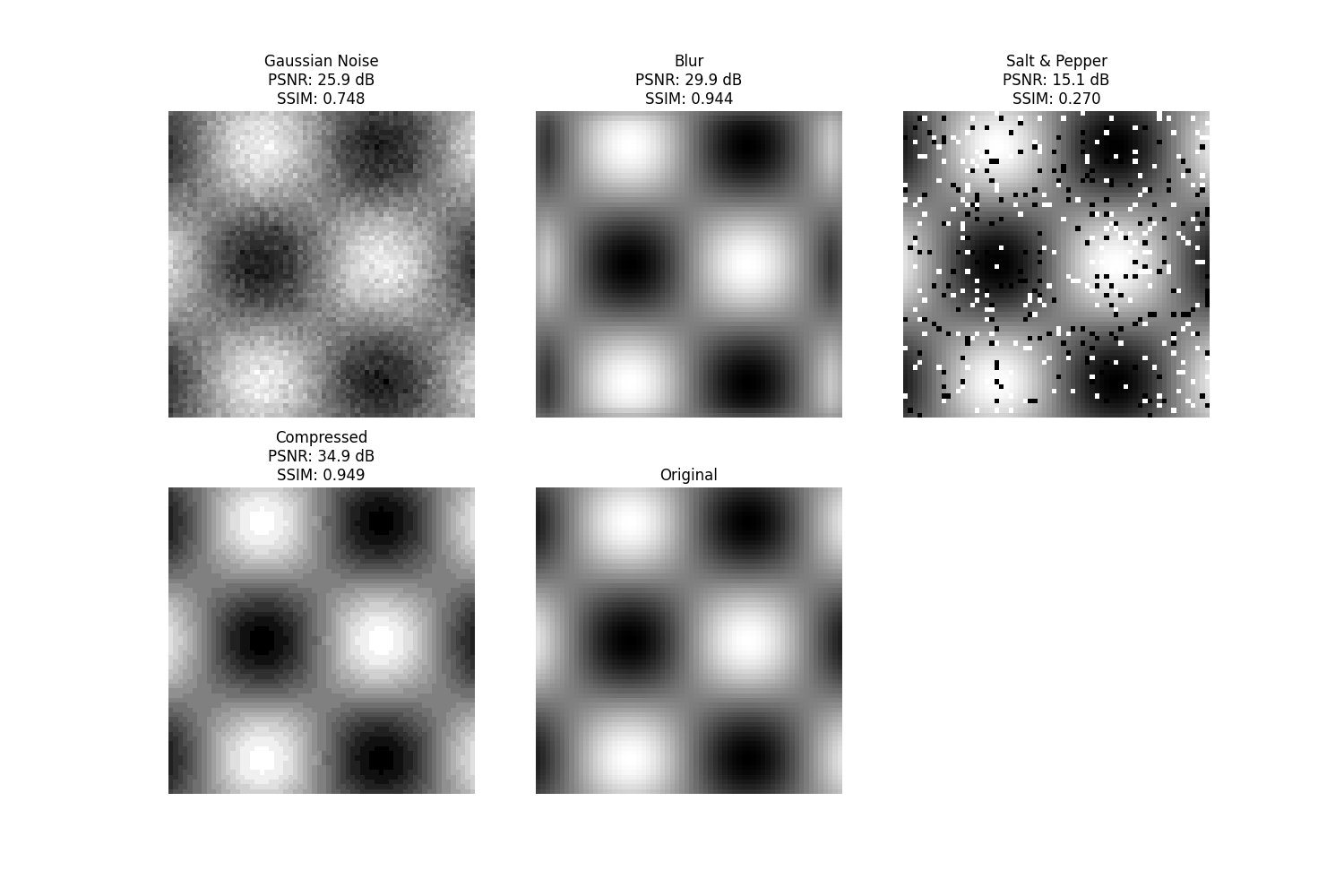
5. Evaluating Multiple Distortions

Compare different types of distortions using composite metrics

# Create different distortions
blur_kernel = 5
blurred_img = torch.nn.functional.avg_pool2d(original_img, kernel_size=blur_kernel, stride=1, padding=blur_kernel // 2)

# Add salt and pepper noise
salt_pepper_img = original_img.clone()
mask = torch.rand_like(salt_pepper_img)
salt_pepper_img[mask < 0.05] = -1.0  # salt
salt_pepper_img[mask > 0.95] = 1.0  # pepper

# Compression effect (simulate with quantization)
compression_levels = 8
compressed_img = torch.round(original_img * compression_levels) / compression_levels

# Evaluate all distortions
distorted_images = {"Gaussian Noise": noisy_img, "Blur": blurred_img, "Salt & Pepper": salt_pepper_img, "Compressed": compressed_img}

# Compute metrics for each distortion
results = {}
for name, img in distorted_images.items():
    results[name] = img_quality_metric(img, original_img)

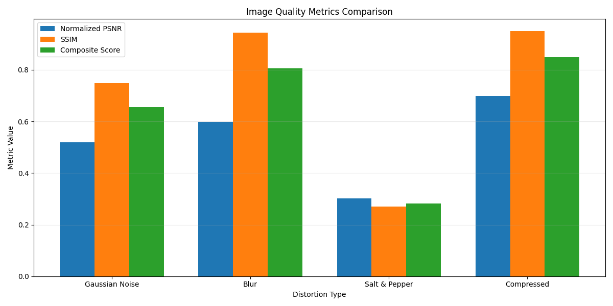
# Visualize all images and metrics
plt.figure(figsize=(15, 10))

# Plot images
for i, (name, img) in enumerate(distorted_images.items()):
    plt.subplot(2, 3, i + 1)
    plt.imshow(img[0, 0].numpy(), cmap="gray")
    plt.title(f'{name}\nPSNR: {results[name]["PSNR"].item():.1f} dB\nSSIM: {results[name]["SSIM"].item():.3f}')
    plt.axis("off")

# Add original image
plt.subplot(2, 3, 5)
plt.imshow(original_img[0, 0].numpy(), cmap="gray")
plt.title("Original")
plt.axis("off")

# Plot metrics comparison
plt.figure(figsize=(12, 6))

# Prepare data for bar chart
names = list(results.keys())
psnr_values = [results[name]["PSNR_normalized"].item() for name in names]
ssim_values = [results[name]["SSIM"].item() for name in names]
composite_values = [results[name]["weighted_score"].item() for name in names]

# Plot as grouped bar chart
x = np.arange(len(names))
width = 0.25

plt.bar(x - width, psnr_values, width, label="Normalized PSNR")
plt.bar(x, ssim_values, width, label="SSIM")
plt.bar(x + width, composite_values, width, label="Composite Score")

plt.xlabel("Distortion Type")
plt.ylabel("Metric Value")
plt.title("Image Quality Metrics Comparison")
plt.xticks(x, names)
plt.legend()
plt.grid(axis="y", alpha=0.3)
plt.tight_layout()
plt.show()

• 
• 

Conclusion

This example demonstrated:

1. Creating and using composite metrics to evaluate multiple aspects of performance

2. Combining metrics with different scales through normalization

3. Applying custom weights to emphasize metrics according to application needs

4. Visualizing trade-offs between different metrics

5. Using composite metrics to compare different types of distortions

Composite metrics are particularly useful when:

• Multiple factors contribute to overall system quality

• Different metrics capture complementary aspects of performance

• Applications require balancing competing objectives

• Standard metrics alone don’t align with specific use case requirements