Note
Go to the end to download the full example code. or to run this example in your browser via Binder
Creating Custom Metrics
This example demonstrates how to create custom metrics by extending the BaseMetric class in the Kaira library. Custom metrics allow you to implement specialized performance measurements for your particular communication system requirements.
import matplotlib.pyplot as plt
Imports and Setup
import numpy as np
import torch

from kaira.metrics import BaseMetric
from kaira.metrics.signal import BER
from kaira.utils import snr_to_noise_power

# Set random seed for reproducibility
torch.manual_seed(42)
np.random.seed(42)
1. Creating a Simple Custom Metric
Start with a basic custom metric that implements error-free-bits ratio
class ErrorFreeBitsRatio(BaseMetric):
    """Custom metric measuring the ratio of error-free bits.

    This is essentially 1 - BER, but demonstrates how to create a basic custom metric.
    """

    def __init__(self, name=None):
        super().__init__(name=name or "ErrorFreeBitsRatio")

    def forward(self, y_pred, y_true):
        """Calculate the ratio of error-free bits.

        Args:
            y_pred (torch.Tensor): Predicted bits (0s and 1s)
            y_true (torch.Tensor): True bits (0s and 1s)

        Returns:
            torch.Tensor: Ratio of bits that are error-free (1 - BER)
        """
        # Number of matching bits
        matching = (y_pred == y_true).float()

        # Calculate ratio
        return torch.mean(matching)


# Test our custom metric
n_bits = 1000
true_bits = torch.randint(0, 2, (1, n_bits))
error_rate = 0.05
errors = torch.rand(1, n_bits) < error_rate
received_bits = torch.logical_xor(true_bits, errors).int()

# Initialize and test our metrics
ber_metric = BER()
efb_metric = ErrorFreeBitsRatio()

ber_value = ber_metric(received_bits, true_bits)
efb_value = efb_metric(received_bits, true_bits)

print(f"BER: {ber_value.item():.5f}")
print(f"Error-Free Bits Ratio: {efb_value.item():.5f}")
print(f"Verification: 1 - BER = {1 - ber_value.item():.5f}")
BER: 0.04000
Error-Free Bits Ratio: 0.96000
Verification: 1 - BER = 0.96000
2. Creating a Parameterized Custom Metric
Implement a custom BER metric with configurable decision thresholds
class AdaptiveThresholdBER(BaseMetric):
    """BER metric with adaptive thresholding based on signal statistics."""

    def __init__(self, threshold_factor=1.0, name=None):
        """Initialize the adaptive threshold BER metric.

        Args:
            threshold_factor (float): Factor to multiply the midpoint threshold
            name (str, optional): Name of the metric
        """
        super().__init__(name=name or f"AdaptiveThresholdBER(factor={threshold_factor})")
        self.threshold_factor = threshold_factor

    def forward(self, y_pred, y_true):
        """Calculate BER with adaptive thresholding.

        Args:
            y_pred (torch.Tensor): Predicted soft bits (real values)
            y_true (torch.Tensor): True bits (0s and 1s)

        Returns:
            torch.Tensor: Bit error rate
        """
        # Use statistics to determine threshold (assuming binary signaling)
        if y_pred.min() < y_pred.max():  # Ensure non-constant input
            # Compute midpoint between min and max
            midpoint = (y_pred.min() + y_pred.max()) / 2
            # Apply threshold factor
            threshold = midpoint * self.threshold_factor
        else:
            threshold = 0.5  # Default if all values are the same

        # Apply threshold
        binary_pred = (y_pred > threshold).int()

        # Calculate number of bit errors
        errors = torch.logical_xor(binary_pred, y_true.int()).float()

        # Return average error rate
        return torch.mean(errors)
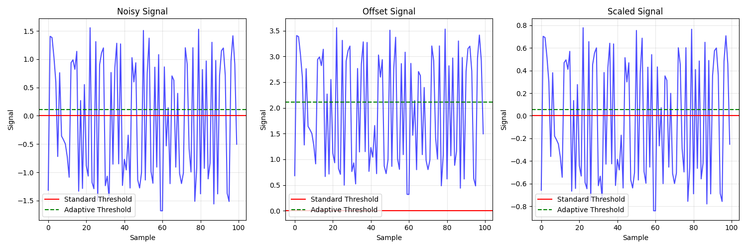
Test the adaptive threshold metric Create a noisy signal with 0s and 1s represented as -1 and +1 with noise
signal_power = 1.0
snr_db = 10
noise_power = snr_to_noise_power(signal_power, snr_db)

# Generate clean signal: -1 for bit 0, +1 for bit 1
true_bits = torch.randint(0, 2, (1, n_bits))
clean_signal = 2 * true_bits.float() - 1  # Map 0->-1, 1->+1

# Add noise
noise = torch.sqrt(torch.tensor(noise_power)) * torch.randn_like(clean_signal)
noisy_signal = clean_signal + noise

# Shift and scale to create a signal with different midpoint
offset_signal = noisy_signal + 2.0  # Shift by 2
scaled_signal = noisy_signal * 0.5  # Scale by 0.5

# Test different threshold factors
threshold_factors = [0.8, 1.0, 1.2]
standard_ber = BER()

print("\nAdaptive Threshold BER Results:")
print(f"Standard BER (noisy): {standard_ber((noisy_signal > 0).int(), true_bits).item():.5f}")
print(f"Standard BER (offset): {standard_ber((offset_signal > 0).int(), true_bits).item():.5f}")
print(f"Standard BER (scaled): {standard_ber((scaled_signal > 0).int(), true_bits).item():.5f}")

for factor in threshold_factors:
    adaptive_ber = AdaptiveThresholdBER(threshold_factor=factor)
    print(f"\nThreshold Factor = {factor}:")
    print(f"Adaptive BER (noisy): {adaptive_ber(noisy_signal, true_bits).item():.5f}")
    print(f"Adaptive BER (offset): {adaptive_ber(offset_signal, true_bits).item():.5f}")
    print(f"Adaptive BER (scaled): {adaptive_ber(scaled_signal, true_bits).item():.5f}")
/home/runner/work/kaira/kaira/examples/metrics/plot_custom_metrics.py:137: UserWarning: To copy construct from a tensor, it is recommended to use sourceTensor.detach().clone() or sourceTensor.detach().clone().requires_grad_(True), rather than torch.tensor(sourceTensor).
  noise = torch.sqrt(torch.tensor(noise_power)) * torch.randn_like(clean_signal)

Adaptive Threshold BER Results:
Standard BER (noisy): 0.00000
Standard BER (offset): 0.50100
Standard BER (scaled): 0.00000

Threshold Factor = 0.8:
Adaptive BER (noisy): 0.00000
Adaptive BER (offset): 0.00800
Adaptive BER (scaled): 0.00000

Threshold Factor = 1.0:
Adaptive BER (noisy): 0.00000
Adaptive BER (offset): 0.00000
Adaptive BER (scaled): 0.00000

Threshold Factor = 1.2:
Adaptive BER (noisy): 0.00000
Adaptive BER (offset): 0.03400
Adaptive BER (scaled): 0.00000
Visualize signals and thresholds
plt.figure(figsize=(15, 5))

# Sample size for visualization
sample_size = 100
samples = np.arange(sample_size)

# Noisy signal
plt.subplot(1, 3, 1)
plt.plot(samples, noisy_signal[0, :sample_size], "b-", alpha=0.7)
plt.axhline(y=0, color="r", linestyle="-", label="Standard Threshold")
plt.axhline(y=noisy_signal.min().item() + (noisy_signal.max() - noisy_signal.min()).item() / 2, color="g", linestyle="--", label="Adaptive Threshold")
plt.grid(True, alpha=0.3)
plt.xlabel("Sample")
plt.ylabel("Signal")
plt.title("Noisy Signal")
plt.legend()

# Offset signal
plt.subplot(1, 3, 2)
plt.plot(samples, offset_signal[0, :sample_size], "b-", alpha=0.7)
plt.axhline(y=0, color="r", linestyle="-", label="Standard Threshold")
plt.axhline(y=offset_signal.min().item() + (offset_signal.max() - offset_signal.min()).item() / 2, color="g", linestyle="--", label="Adaptive Threshold")
plt.grid(True, alpha=0.3)
plt.xlabel("Sample")
plt.ylabel("Signal")
plt.title("Offset Signal")
plt.legend()

# Scaled signal
plt.subplot(1, 3, 3)
plt.plot(samples, scaled_signal[0, :sample_size], "b-", alpha=0.7)
plt.axhline(y=0, color="r", linestyle="-", label="Standard Threshold")
plt.axhline(y=scaled_signal.min().item() + (scaled_signal.max() - scaled_signal.min()).item() / 2, color="g", linestyle="--", label="Adaptive Threshold")
plt.grid(True, alpha=0.3)
plt.xlabel("Sample")
plt.ylabel("Signal")
plt.title("Scaled Signal")
plt.legend()

plt.tight_layout()
plt.show()
3. Creating a More Complex Custom Metric
Implement a weighted error metric where errors in certain positions are considered more serious
class WeightedBER(BaseMetric):
    """BER metric with position-based weighting."""

    def __init__(self, weight_pattern="linear", name=None):
        """Initialize the weighted BER metric.

        Args:
            weight_pattern (str or torch.Tensor): Pattern for position weights:
                'linear': Linear weights (earlier bits more important)
                'alternating': Alternate between more and less important bits
                torch.Tensor: Custom weight pattern
            name (str, optional): Name of the metric
        """
        super().__init__(name=name or f"WeightedBER({weight_pattern})")
        self.weight_pattern = weight_pattern

    def _get_weights(self, length):
        """Generate weights based on the specified pattern.

        Args:
            length (int): Length of the bit sequence

        Returns:
            torch.Tensor: Weight tensor
        """
        if isinstance(self.weight_pattern, torch.Tensor):
            # Use provided weights, repeating if necessary
            pattern_length = self.weight_pattern.numel()
            repeats = (length + pattern_length - 1) // pattern_length
            weights = self.weight_pattern.repeat(repeats)[:length]
            return weights

        elif self.weight_pattern == "linear":
            # Linear weights: earlier bits are more important
            return torch.linspace(1.0, 0.1, length)

        elif self.weight_pattern == "alternating":
            # Alternating weights: even positions more important than odd
            weights = torch.ones(length)
            weights[::2] = 2.0  # Even positions have weight 2
            weights[1::2] = 0.5  # Odd positions have weight 0.5
            return weights

        else:
            # Default: uniform weights
            return torch.ones(length)

    def forward(self, y_pred, y_true):
        """Calculate weighted BER.

        Args:
            y_pred (torch.Tensor): Predicted bits (0s and 1s)
            y_true (torch.Tensor): True bits (0s and 1s)

        Returns:
            torch.Tensor: Weighted bit error rate
        """
        # Get weights
        batch_size, seq_length = y_true.shape
        weights = self._get_weights(seq_length).to(y_true.device)

        # Calculate errors
        errors = torch.logical_xor(y_pred.int(), y_true.int()).float()

        # Apply weights
        weighted_errors = errors * weights.unsqueeze(0)

        # Return weighted average
        return torch.sum(weighted_errors) / torch.sum(weights)
Test the weighted BER metric
# Generate test data
n_bits = 1000
true_bits = torch.randint(0, 2, (1, n_bits))
# Create errors with higher concentration at the beginning
error_prob = torch.linspace(0.1, 0.01, n_bits)  # Error prob decreases linearly
errors = torch.rand(1, n_bits) < error_prob
received_bits = torch.logical_xor(true_bits, errors).int()

# Initialize metrics
standard_ber = BER()
linear_weighted_ber = WeightedBER(weight_pattern="linear")
alternating_weighted_ber = WeightedBER(weight_pattern="alternating")
custom_weights = torch.ones(10)
custom_weights[0:3] = 5.0  # First 3 positions have weight 5
custom_weighted_ber = WeightedBER(weight_pattern=custom_weights)

# Compute BER values
std_ber_value = standard_ber(received_bits, true_bits).item()
linear_ber_value = linear_weighted_ber(received_bits, true_bits).item()
alternating_ber_value = alternating_weighted_ber(received_bits, true_bits).item()
custom_ber_value = custom_weighted_ber(received_bits, true_bits).item()

print("\nWeighted BER Results:")
print(f"Standard BER: {std_ber_value:.5f}")
print(f"Linear Weighted BER: {linear_ber_value:.5f}")
print(f"Alternating Weighted BER: {alternating_ber_value:.5f}")
print(f"Custom Weighted BER: {custom_ber_value:.5f}")
Weighted BER Results:
Standard BER: 0.05100
Linear Weighted BER: 0.06034
Alternating Weighted BER: 0.04800
Custom Weighted BER: 0.05045
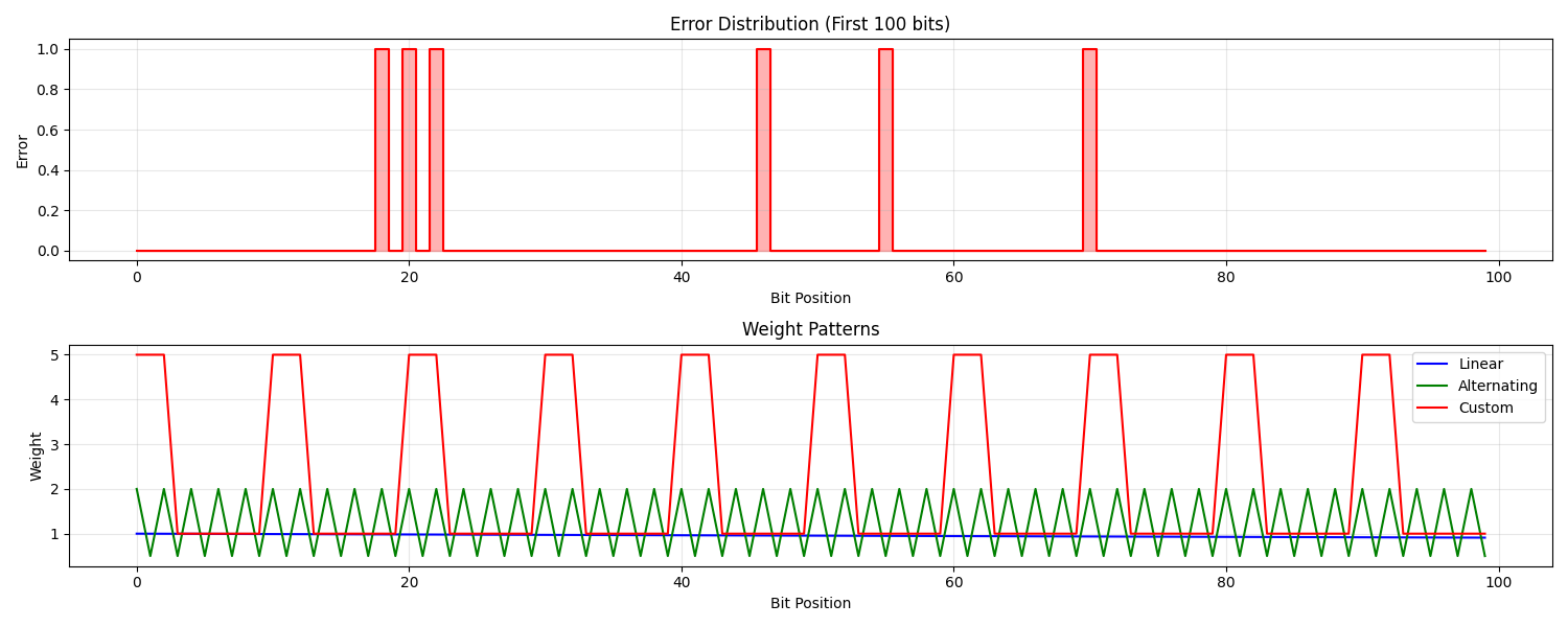
Visualize the weights and error distribution
plt.figure(figsize=(15, 6))

# Plot the first 100 samples for visibility
sample_size = 100

# Plot the error distribution
plt.subplot(2, 1, 1)
plt.step(range(sample_size), errors[0, :sample_size].numpy(), "r-", where="mid")
plt.fill_between(range(sample_size), errors[0, :sample_size].numpy(), step="mid", alpha=0.3, color="r")
plt.grid(True, alpha=0.3)
plt.xlabel("Bit Position")
plt.ylabel("Error")
plt.title("Error Distribution (First 100 bits)")

# Plot the weights
plt.subplot(2, 1, 2)
plt.plot(range(sample_size), linear_weighted_ber._get_weights(n_bits)[:sample_size], "b-", label="Linear")
plt.plot(range(sample_size), alternating_weighted_ber._get_weights(n_bits)[:sample_size], "g-", label="Alternating")

# Plot custom weights (repeat pattern as needed)
custom_pattern = custom_weights.repeat((sample_size + 9) // 10)[:sample_size]
plt.plot(range(sample_size), custom_pattern, "r-", label="Custom")

plt.grid(True, alpha=0.3)
plt.xlabel("Bit Position")
plt.ylabel("Weight")
plt.title("Weight Patterns")
plt.legend()

plt.tight_layout()
plt.show()
4. Application-Specific Custom Metric
Create a custom metric for evaluating the Quality of Service (QoS) of a system
class QualityOfServiceMetric(BaseMetric):
    """Custom metric for evaluating overall Quality of Service.

    Combines multiple factors: error rate, latency, and throughput.
    """

    def __init__(self, error_weight=0.4, latency_weight=0.3, throughput_weight=0.3, name=None):
        """Initialize the QoS metric.

        Args:
            error_weight (float): Weight for error rate (default: 0.4)
            latency_weight (float): Weight for latency (default: 0.3)
            throughput_weight (float): Weight for throughput (default: 0.3)
            name (str, optional): Name of the metric
        """
        super().__init__(name=name or "QualityOfService")
        self.error_weight = error_weight
        self.latency_weight = latency_weight
        self.throughput_weight = throughput_weight

    def forward(self, error_rate, latency_ms, throughput_mbps):
        """Calculate QoS score.

        Args:
            error_rate (torch.Tensor): Error rate (lower is better)
            latency_ms (torch.Tensor): Latency in milliseconds (lower is better)
            throughput_mbps (torch.Tensor): Throughput in Mbps (higher is better)

        Returns:
            torch.Tensor: QoS score (higher is better)
        """
        # Normalize each parameter to [0,1] range where 1 is best
        # For error_rate and latency, lower is better, so use 1 - normalized_value
        # For throughput, higher is better

        # Assuming reasonable ranges for the parameters:
        # Error rate: [0, 0.1] (0% to 10%)
        # Latency: [1, 100] ms
        # Throughput: [1, 1000] Mbps

        # Clip to ensure values are within expected bounds
        error_rate_clipped = torch.clamp(error_rate, 0.0, 0.1)
        latency_clipped = torch.clamp(latency_ms, 1.0, 100.0)
        throughput_clipped = torch.clamp(throughput_mbps, 1.0, 1000.0)

        # Normalize
        norm_error = 1.0 - (error_rate_clipped / 0.1)  # 0 error -> 1, 10% error -> 0
        norm_latency = 1.0 - (torch.log10(latency_clipped) / torch.log10(torch.tensor(100.0)))  # 1ms -> 1, 100ms -> 0
        norm_throughput = torch.log10(throughput_clipped) / torch.log10(torch.tensor(1000.0))  # 1Mbps -> 0, 1000Mbps -> 1

        # Weighted combination
        qos_score = self.error_weight * norm_error + self.latency_weight * norm_latency + self.throughput_weight * norm_throughput

        return qos_score
Test the QoS metric
qos_metric = QualityOfServiceMetric()

# Create a range of test values
error_rates = torch.tensor([[0.001, 0.01, 0.05]])
latencies = torch.tensor([[5.0, 20.0, 50.0]])
throughputs = torch.tensor([[100.0, 50.0, 10.0]])

# Calculate QoS for each scenario
qos_scores = []
for i in range(3):
    score = qos_metric(error_rates[:, i : i + 1], latencies[:, i : i + 1], throughputs[:, i : i + 1])
    qos_scores.append(score.item())

# Display results
scenarios = ["Good", "Average", "Poor"]
print("\nQuality of Service Results:")
print(f"{'Scenario':<10} {'Error Rate':<15} {'Latency (ms)':<15} {'Throughput (Mbps)':<20} {'QoS Score':<10}")
print("-" * 70)
for i in range(3):
    print(f"{scenarios[i]:<10} {error_rates[0,i]:.5f}{'':<9} {latencies[0,i]:<15.1f} {throughputs[0,i]:<20.1f} {qos_scores[i]:.5f}")
Quality of Service Results:
Scenario Error Rate Latency (ms) Throughput (Mbps) QoS Score
----------------------------------------------------------------------
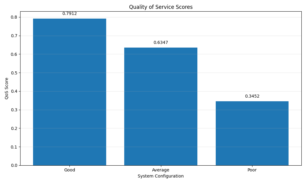
Good 0.00100 5.0 100.0 0.79115
Average 0.01000 20.0 50.0 0.63474
Poor 0.05000 50.0 10.0 0.34515
Visualize the QoS scores for different configurations
plt.figure(figsize=(10, 6))
plt.bar(scenarios, qos_scores)
plt.grid(axis="y", alpha=0.3)
plt.xlabel("System Configuration")
plt.ylabel("QoS Score")
plt.title("Quality of Service Scores")

# Add value labels above bars
for i, score in enumerate(qos_scores):
    plt.text(i, score + 0.02, f"{score:.4f}", ha="center")

plt.tight_layout()
plt.show()
5. Metric that Implements a Communication Standard
Implement a custom metric that follows a communications standard specification
class MeanOpinionScore(BaseMetric):
    """Mean Opinion Score (MOS) metric for voice quality assessment.

    Implements a simplified version of the E-model (ITU-T G.107) to estimate user satisfaction with
    voice quality based on technical parameters.
    """

    def __init__(self, name=None):
        """Initialize the MOS metric."""
        super().__init__(name=name or "MeanOpinionScore")

    def _calculate_r_factor(self, latency_ms, packet_loss_percent, jitter_ms):
        """Calculate the R-factor according to a simplified E-model.

        Args:
            latency_ms (torch.Tensor): One-way latency in milliseconds
            packet_loss_percent (torch.Tensor): Packet loss percentage (0-100)
            jitter_ms (torch.Tensor): Jitter in milliseconds

        Returns:
            torch.Tensor: R-factor (0-100)
        """
        # Simplified version of the E-model
        # R = 100 - Id - Ie - Io + Is

        # Start with maximum quality
        r = torch.tensor(100.0).to(latency_ms.device)

        # Impairment due to delay (Id)
        id_factor = torch.zeros_like(latency_ms)

        # Mild impairment for delay > 150ms, severe for > 300ms
        delay_mask = latency_ms > 150.0
        id_factor = torch.where(delay_mask, 0.02 * (latency_ms - 150.0), id_factor)

        # Additional penalty for delays > 300ms
        severe_delay_mask = latency_ms > 300.0
        id_factor = torch.where(severe_delay_mask, id_factor + 0.1 * (latency_ms - 300.0), id_factor)

        # Impairment due to packet loss (Ie)
        ie_factor = 30.0 * packet_loss_percent / 100.0

        # Impairment due to jitter (simplified)
        io_factor = 15.0 * jitter_ms / 100.0

        # Calculate final R-factor
        r = r - id_factor - ie_factor - io_factor

        # Clamp to valid range
        return torch.clamp(r, 0.0, 100.0)

    def _r_to_mos(self, r_factor):
        """Convert R-factor to MOS score.

        Args:
            r_factor (torch.Tensor): R-factor (0-100)

        Returns:
            torch.Tensor: MOS score (1-5)
        """
        # MOS conversion formula
        # For R < 0: MOS = 1.0
        # For 0 <= R <= 100: MOS = 1 + 0.035*R + R(R-60)(100-R)×7×10^-6
        # For R > 100: MOS = 4.5

        mos = torch.ones_like(r_factor)

        # Apply formula for valid R range
        valid_mask = (r_factor >= 0.0) & (r_factor <= 100.0)
        mos = torch.where(valid_mask, 1.0 + 0.035 * r_factor + r_factor * (r_factor - 60.0) * (100.0 - r_factor) * 7.0e-6, mos)

        # Cap at 4.5 for R > 100
        high_mask = r_factor > 100.0
        mos = torch.where(high_mask, torch.tensor(4.5).to(r_factor.device), mos)

        return mos

    def forward(self, latency_ms, packet_loss_percent, jitter_ms):
        """Calculate Mean Opinion Score (MOS).

        Args:
            latency_ms (torch.Tensor): One-way latency in milliseconds
            packet_loss_percent (torch.Tensor): Packet loss percentage (0-100)
            jitter_ms (torch.Tensor): Jitter in milliseconds

        Returns:
            torch.Tensor: MOS score (1-5)
        """
        r_factor = self._calculate_r_factor(latency_ms, packet_loss_percent, jitter_ms)
        mos = self._r_to_mos(r_factor)
        return mos
Test the MOS metric
mos_metric = MeanOpinionScore()

# Create a range of test values
latencies = torch.tensor([50.0, 150.0, 250.0, 350.0])
packet_losses = torch.tensor([0.0, 1.0, 3.0, 10.0])
jitters = torch.tensor([5.0, 20.0, 50.0, 100.0])

# Calculate MOS for different combinations
print("\nMean Opinion Score (MOS) Results:")
print(f"{'Latency (ms)':<15} {'Packet Loss (%)':<15} {'Jitter (ms)':<15} {'R-Factor':<15} {'MOS':<10} {'Quality':<15}")
print("-" * 85)

for latency in latencies:
    for loss in packet_losses:
        for jitter in jitters:
            # Convert to 2D tensors for the metric
            lat_tensor = latency.unsqueeze(0).unsqueeze(0)
            loss_tensor = loss.unsqueeze(0).unsqueeze(0)
            jitter_tensor = jitter.unsqueeze(0).unsqueeze(0)

            # Calculate R-factor and MOS
            r_factor = mos_metric._calculate_r_factor(lat_tensor, loss_tensor, jitter_tensor)
            mos = mos_metric(lat_tensor, loss_tensor, jitter_tensor)

            # Determine quality category
            quality = "Unknown"
            if mos >= 4.3:
                quality = "Excellent"
            elif mos >= 4.0:
                quality = "Good"
            elif mos >= 3.6:
                quality = "Fair"
            elif mos >= 3.1:
                quality = "Poor"
            else:
                quality = "Bad"

            print(f"{latency.item():<15} {loss.item():<15} {jitter.item():<15} {r_factor.item():<15.1f} {mos.item():<10.2f} {quality:<15}")
Mean Opinion Score (MOS) Results:
Latency (ms)    Packet Loss (%) Jitter (ms)     R-Factor        MOS        Quality
-------------------------------------------------------------------------------------
50.0            0.0             5.0             99.2            4.49       Excellent
50.0            0.0             20.0            97.0            4.47       Excellent
50.0            0.0             50.0            92.5            4.40       Excellent
50.0            0.0             100.0           85.0            4.20       Good
50.0            1.0             5.0             98.9            4.49       Excellent
50.0            1.0             20.0            96.7            4.47       Excellent
50.0            1.0             50.0            92.2            4.39       Excellent
50.0            1.0             100.0           84.7            4.19       Good
50.0            3.0             5.0             98.3            4.49       Excellent
50.0            3.0             20.0            96.1            4.46       Excellent
50.0            3.0             50.0            91.6            4.38       Excellent
50.0            3.0             100.0           84.1            4.17       Good
50.0            10.0            5.0             96.2            4.46       Excellent
50.0            10.0            20.0            94.0            4.42       Excellent
50.0            10.0            50.0            89.5            4.33       Excellent
50.0            10.0            100.0           82.0            4.10       Good
150.0           0.0             5.0             99.2            4.49       Excellent
150.0           0.0             20.0            97.0            4.47       Excellent
150.0           0.0             50.0            92.5            4.40       Excellent
150.0           0.0             100.0           85.0            4.20       Good
150.0           1.0             5.0             98.9            4.49       Excellent
150.0           1.0             20.0            96.7            4.47       Excellent
150.0           1.0             50.0            92.2            4.39       Excellent
150.0           1.0             100.0           84.7            4.19       Good
150.0           3.0             5.0             98.3            4.49       Excellent
150.0           3.0             20.0            96.1            4.46       Excellent
150.0           3.0             50.0            91.6            4.38       Excellent
150.0           3.0             100.0           84.1            4.17       Good
150.0           10.0            5.0             96.2            4.46       Excellent
150.0           10.0            20.0            94.0            4.42       Excellent
150.0           10.0            50.0            89.5            4.33       Excellent
150.0           10.0            100.0           82.0            4.10       Good
250.0           0.0             5.0             97.2            4.47       Excellent
250.0           0.0             20.0            95.0            4.44       Excellent
250.0           0.0             50.0            90.5            4.35       Excellent
250.0           0.0             100.0           83.0            4.13       Good
250.0           1.0             5.0             96.9            4.47       Excellent
250.0           1.0             20.0            94.7            4.44       Excellent
250.0           1.0             50.0            90.2            4.34       Excellent
250.0           1.0             100.0           82.7            4.12       Good
250.0           3.0             5.0             96.3            4.46       Excellent
250.0           3.0             20.0            94.1            4.43       Excellent
250.0           3.0             50.0            89.6            4.33       Excellent
250.0           3.0             100.0           82.1            4.10       Good
250.0           10.0            5.0             94.2            4.43       Excellent
250.0           10.0            20.0            92.0            4.38       Excellent
250.0           10.0            50.0            87.5            4.27       Good
250.0           10.0            100.0           80.0            4.02       Good
350.0           0.0             5.0             90.2            4.35       Excellent
350.0           0.0             20.0            88.0            4.29       Good
350.0           0.0             50.0            83.5            4.15       Good
350.0           0.0             100.0           76.0            3.86       Fair
350.0           1.0             5.0             89.9            4.34       Excellent
350.0           1.0             20.0            87.7            4.28       Good
350.0           1.0             50.0            83.2            4.14       Good
350.0           1.0             100.0           75.7            3.85       Fair
350.0           3.0             5.0             89.3            4.32       Excellent
350.0           3.0             20.0            87.1            4.26       Good
350.0           3.0             50.0            82.6            4.12       Good
350.0           3.0             100.0           75.1            3.83       Fair
350.0           10.0            5.0             87.2            4.27       Good
350.0           10.0            20.0            85.0            4.20       Good
350.0           10.0            50.0            80.5            4.04       Good
350.0           10.0            100.0           73.0            3.73       Fair
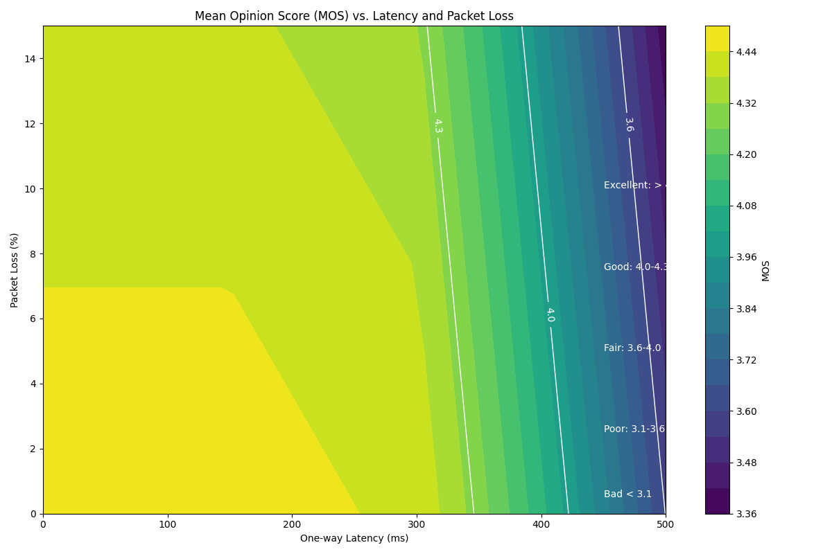
Visualize the effect of parameters on MOS Create a grid of latency and packet loss values
latencies = torch.linspace(0, 500, 50)
packet_losses = torch.linspace(0, 15, 50)
lat_grid, loss_grid = torch.meshgrid(latencies, packet_losses, indexing="ij")

# Calculate MOS for each combination (with fixed jitter of 20ms)
mos_values = torch.zeros_like(lat_grid)
for i in range(lat_grid.shape[0]):
    for j in range(lat_grid.shape[1]):
        lat_tensor = lat_grid[i, j].unsqueeze(0).unsqueeze(0)
        loss_tensor = loss_grid[i, j].unsqueeze(0).unsqueeze(0)
        jitter_tensor = torch.tensor([[20.0]])

        mos_values[i, j] = mos_metric(lat_tensor, loss_tensor, jitter_tensor).item()

# Plot the results
plt.figure(figsize=(12, 8))
contour = plt.contourf(lat_grid.numpy(), loss_grid.numpy(), mos_values.numpy(), 20, cmap="viridis")
plt.colorbar(contour, label="MOS")
plt.xlabel("One-way Latency (ms)")
plt.ylabel("Packet Loss (%)")
plt.title("Mean Opinion Score (MOS) vs. Latency and Packet Loss")

# Add contour lines for specific MOS values
contour_lines = plt.contour(lat_grid.numpy(), loss_grid.numpy(), mos_values.numpy(), levels=[1.0, 2.0, 3.0, 3.6, 4.0, 4.3], colors="white", linestyles="solid", linewidths=1)
plt.clabel(contour_lines, inline=True, fontsize=10, fmt="%.1f")

# Add quality regions annotation
plt.text(450, 0.5, "Bad < 3.1", color="white", fontsize=10)
plt.text(450, 2.5, "Poor: 3.1-3.6", color="white", fontsize=10)
plt.text(450, 5.0, "Fair: 3.6-4.0", color="white", fontsize=10)
plt.text(450, 7.5, "Good: 4.0-4.3", color="white", fontsize=10)
plt.text(450, 10.0, "Excellent: > 4.3", color="white", fontsize=10)

plt.tight_layout()
plt.show()
Conclusion
This example demonstrated:
How to create custom metrics by extending the BaseMetric class
Creating simple, parameterized, and complex custom metrics
Implementing application-specific metrics for specialized use cases
Creating metrics that implement communication standards
Visualizing metric behavior under different conditions
Key takeaways:
Custom metrics enable specialized evaluation for unique requirements
Parameterized metrics allow flexible adaptation to different scenarios
Position-weighted metrics can prioritize critical data segments
Application-specific metrics can combine multiple factors into a single score
Communication standards can be implemented as metrics for standardized evaluation
Total running time of the script: (0 minutes 1.299 seconds)