Image Quality Metrics

This example demonstrates the image quality metrics available in Kaira, including PSNR (Peak Signal-to-Noise Ratio), SSIM (Structural Similarity Index), MS-SSIM (Multi-Scale SSIM), and LPIPS (Learned Perceptual Image Patch Similarity).

These metrics are particularly useful for: * Evaluating image compression algorithms * Assessing deep learning-based image processing * Quality control in image transmission systems

import os
from pathlib import Path

import matplotlib.pyplot as plt

First, let’s import the necessary modules

import torch
import torchvision.transforms as T
from PIL import Image

from kaira.metrics.image.lpips import LearnedPerceptualImagePatchSimilarity
from kaira.metrics.image.psnr import PeakSignalNoiseRatio
from kaira.metrics.image.ssim import MultiScaleSSIM, StructuralSimilarityIndexMeasure

# Sample images path - handle both script and interactive environments
try:
    SAMPLE_IMAGES_DIR = Path(__file__).parent / "sample_images"
except NameError:
    # Fallback for interactive environments
    SAMPLE_IMAGES_DIR = Path.cwd() / "sample_images"


def load_sample_images(num_images=4):
    """Load sample test images for demonstration."""
    transform = T.Compose(
        [
            T.Resize((256, 256)),
            T.ToTensor(),
        ]
    )

    images = []
    for img_file in sorted(SAMPLE_IMAGES_DIR.glob("*.png"))[:num_images]:
        # Handle both PNG and TIFF formats
        img = Image.open(str(img_file)).convert("RGB")
        images.append(transform(img))

    return torch.stack(images)


# Ensure test images are available
if not SAMPLE_IMAGES_DIR.exists() or not list(SAMPLE_IMAGES_DIR.glob("*.*")):
    raise RuntimeError("Test images not found. Please run:\n" + str(SAMPLE_IMAGES_DIR) + "\n" + "python scripts/download_test_images.py")

# Load sample images
images = load_sample_images(4)

Create different types of distortions

We’ll create different types of distortions to compare how various metrics assess them

def add_gaussian_noise(image, std=0.1):
    """Add Gaussian noise to image."""
    return image + torch.randn_like(image) * std


def add_salt_pepper_noise(image, prob=0.05):
    """Add salt and pepper noise to image."""
    mask = torch.rand_like(image)
    image = image.clone()
    image[mask < prob / 2] = 0  # salt
    image[mask > 1 - prob / 2] = 1  # pepper
    return image


def blur_image(image, kernel_size=3):
    """Apply Gaussian blur to image."""
    return T.GaussianBlur(kernel_size)(image)


def compress_image(image, quality=10):
    """Simulate JPEG compression artifacts."""
    to_pil = T.ToPILImage()
    to_tensor = T.ToTensor()
    pil_image = to_pil(image)
    # Create a temporary file for compression
    temp_file = "temp.jpg"
    pil_image.save(temp_file, quality=quality)
    try:
        compressed = Image.open(temp_file)
        return to_tensor(compressed)
    finally:
        if os.path.exists(temp_file):
            os.remove(temp_file)


# Create distorted versions
noisy_images = torch.stack([add_gaussian_noise(img) for img in images])
sp_noisy_images = torch.stack([add_salt_pepper_noise(img) for img in images])
blurred_images = torch.stack([blur_image(img) for img in images])
compressed_images = torch.stack([compress_image(img) for img in images])

Initialize metrics

We’ll create individual metrics directly without using the registry

# Initialize metrics manually
psnr = PeakSignalNoiseRatio(data_range=1.0, reduction="mean")  # or PSNR()
ssim = StructuralSimilarityIndexMeasure(data_range=1.0, reduction="mean")  # or SSIM()
ms_ssim = MultiScaleSSIM(data_range=1.0, reduction="mean")  # Add reduction parameter
lpips = LearnedPerceptualImagePatchSimilarity(net_type="alex")  # remove redundant reduction parameter

Downloading: "https://download.pytorch.org/models/alexnet-owt-7be5be79.pth" to /home/runner/.cache/torch/hub/checkpoints/alexnet-owt-7be5be79.pth

  0%|          | 0.00/233M [00:00<?, ?B/s]
  7%|▋         | 15.6M/233M [00:00<00:01, 164MB/s]
 21%|██▏       | 49.8M/233M [00:00<00:00, 278MB/s]
 36%|███▌      | 83.1M/233M [00:00<00:00, 310MB/s]
 51%|█████▏    | 120M/233M [00:00<00:00, 339MB/s]
 66%|██████▌   | 154M/233M [00:00<00:00, 348MB/s]
 82%|████████▏ | 191M/233M [00:00<00:00, 360MB/s]
 97%|█████████▋| 226M/233M [00:00<00:00, 318MB/s]
100%|██████████| 233M/233M [00:00<00:00, 319MB/s]

Evaluate metrics on different distortions

def evaluate_all_metrics(original, distorted):
    """Evaluate all metrics between original and distorted images."""
    return {"PSNR": psnr(distorted, original), "SSIM": ssim(distorted, original), "MS-SSIM": ms_ssim(distorted, original), "LPIPS": lpips(distorted, original)}  # Now returns scalar mean  # Now returns scalar mean  # Now returns scalar mean  # Now returns scalar mean


# Evaluate metrics for each type of distortion
gaussian_metrics = evaluate_all_metrics(images, noisy_images)
sp_metrics = evaluate_all_metrics(images, sp_noisy_images)
blur_metrics = evaluate_all_metrics(images, blurred_images)
compress_metrics = evaluate_all_metrics(images, compressed_images)

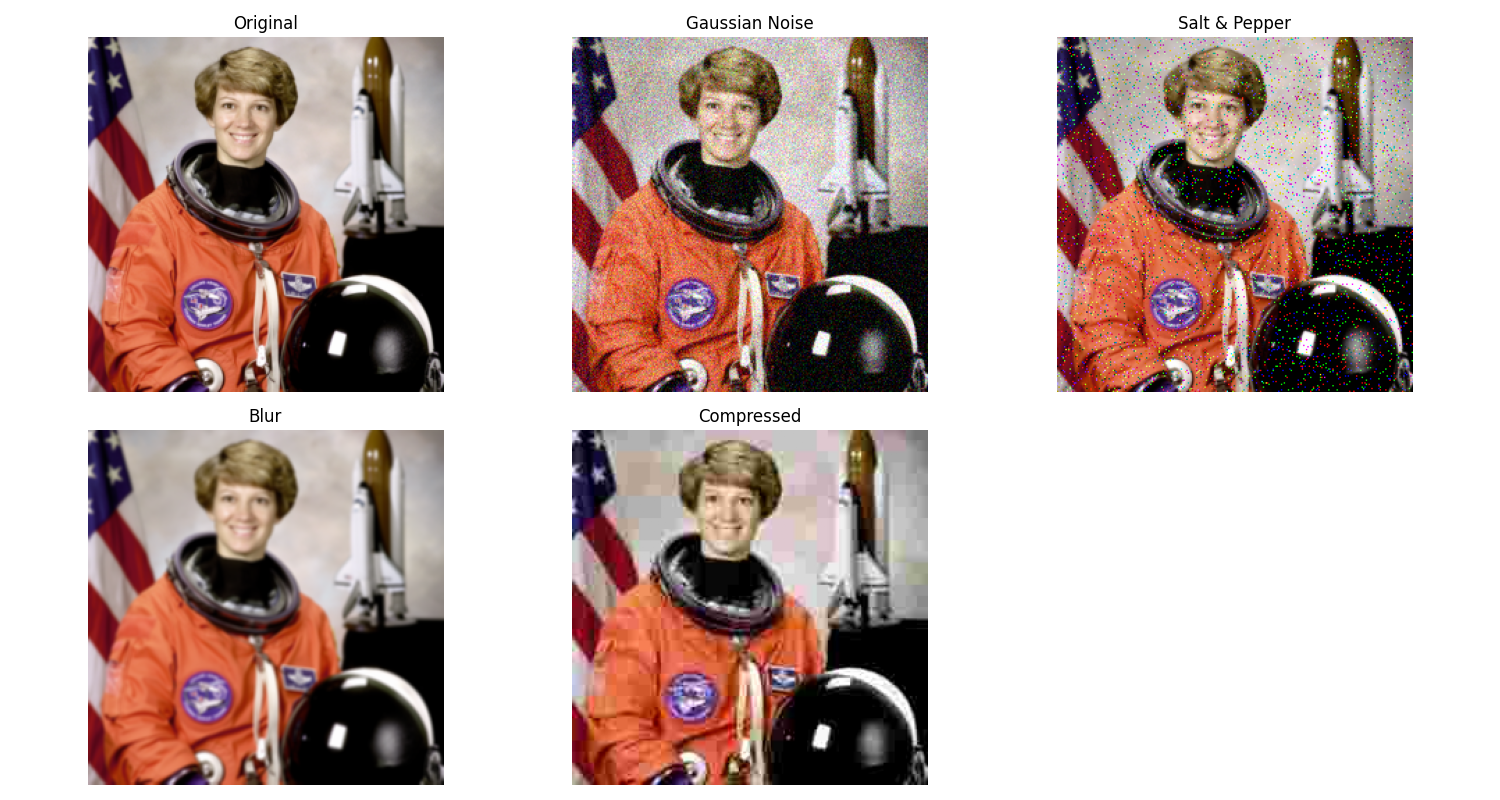
Visualize results

First, let’s look at the distorted images

plt.figure(figsize=(15, 8))
titles = ["Original", "Gaussian Noise", "Salt & Pepper", "Blur", "Compressed"]
all_images = [images, noisy_images, sp_noisy_images, blurred_images, compressed_images]

for i, (title, imgs) in enumerate(zip(titles, all_images)):
    plt.subplot(2, 3, i + 1)
    plt.imshow(imgs[0].permute(1, 2, 0).clip(0, 1))
    plt.title(title)
    plt.axis("off")

plt.tight_layout()
plt.show()

Now let’s compare how different metrics evaluate each distortion type

all_metrics = [gaussian_metrics, sp_metrics, blur_metrics, compress_metrics]

labels = ["Gaussian", "Salt & Pepper", "Blur", "Compression"]

# Create a manual comparison visualization
plt.figure(figsize=(14, 10))

# Plot PSNR values
plt.subplot(2, 2, 1)
psnr_values = [metrics["PSNR"].item() for metrics in all_metrics]  # Convert tensor to Python scalar
plt.bar(labels, psnr_values, color="blue")
plt.xlabel("Distortion Type")
plt.ylabel("PSNR (dB)")
plt.title("PSNR Comparison")
plt.grid(axis="y", alpha=0.3)

# Plot SSIM values
plt.subplot(2, 2, 2)
ssim_values = [metrics["SSIM"].item() for metrics in all_metrics]  # Convert tensor to Python scalar
plt.bar(labels, ssim_values, color="green")
plt.xlabel("Distortion Type")
plt.ylabel("SSIM")
plt.title("SSIM Comparison")
plt.grid(axis="y", alpha=0.3)

# Plot MS-SSIM values
plt.subplot(2, 2, 3)
msssim_values = [metrics["MS-SSIM"].item() for metrics in all_metrics]  # Convert tensor to Python scalar
plt.bar(labels, msssim_values, color="purple")
plt.xlabel("Distortion Type")
plt.ylabel("MS-SSIM")
plt.title("MS-SSIM Comparison")
plt.grid(axis="y", alpha=0.3)

# Plot LPIPS values (lower is better)
plt.subplot(2, 2, 4)
lpips_values = [metrics["LPIPS"].item() for metrics in all_metrics]  # Convert tensor to Python scalar
plt.bar(labels, lpips_values, color="red")
plt.xlabel("Distortion Type")
plt.ylabel("LPIPS (lower is better)")
plt.title("LPIPS Comparison")
plt.grid(axis="y", alpha=0.3)

plt.tight_layout()
plt.show()

Interpreting the Results

The results show how different metrics capture various aspects of image quality:

• PSNR is a simple pixel-level metric that measures absolute differences * Higher values indicate better quality * More sensitive to noise than blurring * May not align well with human perception

• SSIM considers structural information * Values range from -1 to 1 (higher is better) * More tolerant of uniform changes * Better correlation with human perception than PSNR

• MS-SSIM evaluates structural similarity at multiple scales * Similar to SSIM but captures both local and global structures * Often preferred for high-resolution images * Better at detecting blur than basic SSIM

• LPIPS uses deep features to measure perceptual similarity * Lower values indicate better perceptual quality * Trained on human perceptual judgments * Often best matches human quality assessment

Different distortions affect these metrics differently:

• Gaussian noise heavily impacts PSNR but less so SSIM

• Blur might maintain good PSNR but show poor SSIM/MS-SSIM

• LPIPS often identifies perceptually significant distortions that other metrics might miss

For practical applications:

• Use multiple metrics for comprehensive evaluation

• Consider the specific requirements of your application

• LPIPS is recommended when perceptual quality is critical

• PSNR/SSIM are good for optimization objectives due to their mathematical properties