Attention-Feature Module (AFModule)

This example demonstrates the Attention-Feature Module (AFModule), which recalibrates feature maps by explicitly modeling interdependencies between channel state information and input features.

The AFModule allows the same model to be used during training and testing across channels with different signal-to-noise ratios without significant performance degradation. It is particularly useful in wireless communication scenarios where channel conditions vary.

import matplotlib.pyplot as plt
import numpy as np
import torch
import torch.nn as nn

from kaira.channels import AWGNChannel
from kaira.models.base import BaseModel
from kaira.models.components import AFModule

# Set random seed for reproducibility
torch.manual_seed(42)
np.random.seed(42)

Introduction to AFModule

The AFModule is designed to adapt neural network behavior based on channel state information (CSI). It was introduced in [Xu et al., 2021] to help models perform consistently across varying channel conditions. This is especially important for wireless communication systems operating in dynamic environments.

Basic structure of the AFModule: 1. It takes two inputs: feature maps and channel state information 2. It calculates an attention mask based on these inputs 3. The mask is applied to the original feature maps to recalibrate them

Let’s create a simple AFModule and explore its behavior:

# Define parameters
batch_size = 8
N = 64  # Number of feature channels
csi_length = 1  # Length of channel state information

# Create an AFModule
af_module = AFModule(N=N, csi_length=csi_length)
print(f"AFModule structure:\n{af_module}")

AFModule structure:
AFModule(
  (layers): Sequential(
    (0): Linear(in_features=65, out_features=64, bias=True)
    (1): LeakyReLU(negative_slope=0.01)
    (2): Linear(in_features=64, out_features=64, bias=True)
    (3): Sigmoid()
  )
)

Basic Usage with 2D Tensor Input

Let’s first examine how the AFModule works with 2D tensor inputs, which represents the simplest use case.

# Create a 2D input tensor (batch_size, N)
input_2d = torch.randn(batch_size, N)
print(f"Input shape (2D): {input_2d.shape}")

# Create channel state information (CSI) - varies between 0 and 1 for this example
# In practice, this could be SNR values or other channel quality indicators
csi_values = torch.linspace(0.1, 0.9, batch_size).unsqueeze(1)  # Shape: (batch_size, 1)
print(f"CSI values: {csi_values.squeeze().numpy().round(2)}")

# Apply the AFModule
output_2d = af_module(input_2d, csi_values)
print(f"Output shape (2D): {output_2d.shape}")

Input shape (2D): torch.Size([8, 64])
CSI values: [0.1  0.21 0.33 0.44 0.56 0.67 0.79 0.9 ]
Output shape (2D): torch.Size([8, 64])

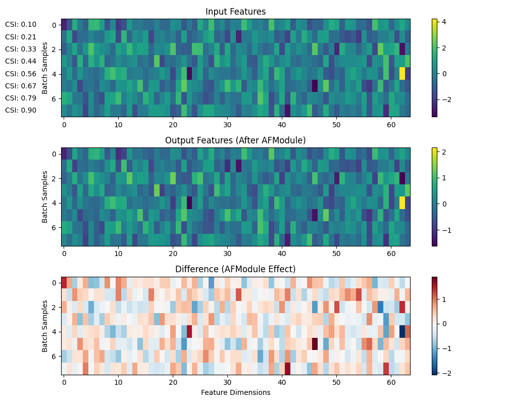
Visualizing the Effect of AFModule on 2D Data

Let’s visualize how different CSI values affect the features

# Create a heatmap visualization function
def visualize_features(input_tensor, output_tensor, csi_values, title):
    """Visualize input and output features along with CSI values."""
    fig, axes = plt.subplots(3, 1, figsize=(10, 8))

    # Plot input features
    im1 = axes[0].imshow(input_tensor.detach().numpy(), aspect="auto", cmap="viridis")
    axes[0].set_title("Input Features")
    axes[0].set_ylabel("Batch Samples")
    plt.colorbar(im1, ax=axes[0])

    # Plot output features
    im2 = axes[1].imshow(output_tensor.detach().numpy(), aspect="auto", cmap="viridis")
    axes[1].set_title("Output Features (After AFModule)")
    axes[1].set_ylabel("Batch Samples")
    plt.colorbar(im2, ax=axes[1])

    # Plot the difference (showing the effect of AFModule)
    difference = output_tensor.detach().numpy() - input_tensor.detach().numpy()
    im3 = axes[2].imshow(difference, aspect="auto", cmap="RdBu_r")
    axes[2].set_title("Difference (AFModule Effect)")
    axes[2].set_ylabel("Batch Samples")
    axes[2].set_xlabel("Feature Dimensions")
    plt.colorbar(im3, ax=axes[2])

    # Add CSI values as text labels
    for i, csi in enumerate(csi_values.squeeze().numpy()):
        axes[0].text(-5, i, f"CSI: {csi:.2f}", ha="right", va="center")

    plt.tight_layout()
    plt.suptitle(title, y=1.02, fontsize=16)
    plt.show()


# Visualize 2D data
visualize_features(input_2d, output_2d, csi_values, "AFModule Effect on 2D Features")

Using AFModule with 4D Tensor Input (Image-like data)

In practice, AFModule is often used with convolutional neural networks where the input is a 4D tensor (batch_size, channels, height, width).

# Create a 4D input tensor (batch_size, channels, height, width)
height, width = 16, 16  # Small image dimensions for visualization
input_4d = torch.randn(batch_size, N, height, width)
print(f"Input shape (4D): {input_4d.shape}")

# Apply the AFModule with the same CSI values
output_4d = af_module(input_4d, csi_values)
print(f"Output shape (4D): {output_4d.shape}")

Input shape (4D): torch.Size([8, 64, 16, 16])
Output shape (4D): torch.Size([8, 64, 16, 16])

Visualizing the Effect on Image-like Data

Let’s visualize a single channel before and after the AFModule

# Choose which channel and sample to visualize
channel_idx = 0
sample_indices = [0, 3, 7]  # Low, medium, and high CSI values

fig, axes = plt.subplots(len(sample_indices), 3, figsize=(12, 3 * len(sample_indices)))

for i, sample_idx in enumerate(sample_indices):
    # Get the input and output for this sample
    input_img = input_4d[sample_idx, channel_idx].detach().numpy()
    output_img = output_4d[sample_idx, channel_idx].detach().numpy()
    difference = output_img - input_img

    # Get the CSI value
    csi_val = csi_values[sample_idx].item()

    # Plot
    im1 = axes[i, 0].imshow(input_img, cmap="viridis")
    axes[i, 0].set_title(f"Input (CSI: {csi_val:.2f})")
    plt.colorbar(im1, ax=axes[i, 0])

    im2 = axes[i, 1].imshow(output_img, cmap="viridis")
    axes[i, 1].set_title("Output (After AFModule)")
    plt.colorbar(im2, ax=axes[i, 1])

    im3 = axes[i, 2].imshow(difference, cmap="RdBu_r")
    axes[i, 2].set_title("Difference")
    plt.colorbar(im3, ax=axes[i, 2])

plt.tight_layout()
plt.suptitle("AFModule Effect on Image Features at Different CSI Values", y=1.02, fontsize=16)
plt.show()

The Role of AFModule in a Real Channel Model

Let’s simulate how AFModule would be used in a real wireless communication scenario with an AWGN channel at different SNR levels.

# Create a simple model with AFModule
class SimpleEncoder(BaseModel):
    """A simple encoder model that incorporates the Attention-Feature Module.

    This encoder processes input data through a linear layer and applies
    the AFModule to dynamically adjust features based on channel conditions
    represented by SNR values.

    Parameters
    ----------
    input_size : int
        The size of the input feature dimension.
    hidden_size : int
        The size of the hidden layer and output feature dimension.
    """

    def __init__(self, input_size, hidden_size):
        super().__init__()
        self.linear = nn.Linear(input_size, hidden_size)
        self.activation = nn.ReLU()
        self.af_module = AFModule(N=hidden_size, csi_length=1)

    def forward(self, x, snr):
        """Forward pass of the encoder.

        Parameters
        ----------
        x : torch.Tensor
            Input tensor of shape (batch_size, input_size).
        snr : torch.Tensor
            Signal-to-noise ratio values represented as a tensor of shape
            (batch_size, 1). These values should be normalized to the range [0, 1].

        Returns
        -------
        torch.Tensor
            Encoded and adaptive feature representation with shape (batch_size, hidden_size).
        """
        x = self.linear(x)
        x = self.activation(x)
        x = self.af_module(x, snr)
        return x


# Create the channel model
channel = AWGNChannel(snr_db=10.0)  # Initialize with a default SNR value

# Create the model
input_size = 32
hidden_size = 64
model = SimpleEncoder(input_size, hidden_size)

# Create input data
input_data = torch.randn(batch_size, input_size)

# Simulate transmission over AWGN channel at different SNR levels
snr_levels = torch.tensor([0, 5, 10, 15, 20, 25]).float()
results = []

for snr in snr_levels:
    # Normalize SNR for the AFModule (assuming SNR is in dB)
    normalized_snr = torch.ones(batch_size, 1) * (snr / 30.0)  # Normalize to [0,1] range

    # Encode the data with AFModule knowing the channel conditions
    encoded = model(input_data, normalized_snr)

    # Pass through the channel with this SNR
    # Create a new channel for each SNR level
    awgn_channel = AWGNChannel(snr_db=snr.item())
    received = awgn_channel(encoded)

    # Store the results
    results.append((snr.item(), encoded.detach(), received.detach()))

Visualizing the Impact of AFModule at Different SNR Levels

Let’s see how the AFModule adapts the encoding based on different SNR levels and how this affects the signal after passing through the channel.

# Visualize the results
fig, axes = plt.subplots(2, len(snr_levels), figsize=(15, 6))

for i, (snr, encoded, received) in enumerate(results):
    # Get the first sample in the batch
    enc_sample = encoded[0].numpy()
    rec_sample = received[0].numpy()

    # Plot
    im1 = axes[0, i].imshow(enc_sample.reshape(8, 8), cmap="viridis")
    axes[0, i].set_title(f"Encoded (SNR: {snr} dB)")

    im2 = axes[1, i].imshow(rec_sample.reshape(8, 8), cmap="viridis")
    axes[1, i].set_title("After Channel")

    if i == 0:
        axes[0, i].set_ylabel("Encoded Signal")
        axes[1, i].set_ylabel("Received Signal")

plt.tight_layout()
plt.suptitle("Effect of AFModule Adaptations at Different SNR Levels", y=1.02, fontsize=16)
plt.show()

Advanced Feature: Dynamic Adaptation

One key feature of AFModule is its ability to dynamically adapt to different input feature sizes. Let’s demonstrate this with a more complex example.

# Create an AFModule with a fixed N value
N_fixed = 64
af_module_fixed = AFModule(N=N_fixed, csi_length=1)

# Create inputs with varying feature dimensions
feature_sizes = [32, 64, 96]
csi_test = torch.ones(1, 1) * 0.5  # Fixed CSI for this test

fig, axes = plt.subplots(len(feature_sizes), 2, figsize=(10, 3 * len(feature_sizes)))

for i, size in enumerate(feature_sizes):
    # Create input with this feature size
    test_input = torch.randn(1, size)

    # Process with the AFModule
    test_output = af_module_fixed(test_input, csi_test)

    # Check shape - should match the input
    print(f"Input size: {size}, Output size: {test_output.shape[1]}")

    # Visualize
    axes[i, 0].bar(range(size), test_input[0].detach().numpy())
    axes[i, 0].set_title(f"Input (Features: {size})")
    axes[i, 0].set_ylim(-3, 3)

    axes[i, 1].bar(range(size), test_output[0].detach().numpy())
    axes[i, 1].set_title("Output after AFModule")
    axes[i, 1].set_ylim(-3, 3)

plt.tight_layout()
plt.suptitle("AFModule Handling Different Feature Sizes", y=1.02, fontsize=16)
plt.show()

Input size: 32, Output size: 32
Input size: 64, Output size: 64
Input size: 96, Output size: 96

Conclusion

In this example, we explored the Attention-Feature Module (AFModule), a component designed to help neural networks adapt to varying channel conditions in wireless communication systems.

Key Points:

• AFModule recalibrates feature maps based on channel state information

• It can work with different input tensor dimensions (2D, 3D, 4D)

• It helps maintain performance across different channel conditions (like varying SNRs)

• The module can adapt to different feature sizes dynamically

The AFModule is particularly useful in deep learning-based communication systems that need to operate reliably in varying channel conditions.

References:

• [Xu et al., 2021]