Original DeepJSCC Model (Bourtsoulatze 2019)

This example demonstrates how to use the original DeepJSCC model from Bourtsoulatze et al. (2019), which pioneered deep learning-based joint source-channel coding for image transmission over wireless channels.

import matplotlib.pyplot as plt

Imports and Setup

import numpy as np
import torch

from kaira.channels import AWGNChannel, FlatFadingChannel
from kaira.constraints import TotalPowerConstraint
from kaira.data.sample_data import load_sample_images
from kaira.metrics.image import PSNR, SSIM
from kaira.models.deepjscc import DeepJSCCModel
from kaira.models.image.bourtsoulatze2019_deepjscc import (
    Bourtsoulatze2019DeepJSCCDecoder,
    Bourtsoulatze2019DeepJSCCEncoder,
)

# Set random seed for reproducibility
torch.manual_seed(42)
np.random.seed(42)

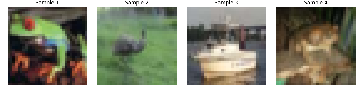
Loading Sample Images

Load sample images from the CIFAR-10 dataset for our demonstration

images, _ = load_sample_images(dataset="cifar10", num_samples=4)
image_size = images.shape[2]  # Should be 32 for CIFAR-10

# Display sample images
plt.figure(figsize=(12, 3))
for i in range(min(4, len(images))):
    plt.subplot(1, 4, i + 1)
    plt.imshow(images[i].permute(1, 2, 0).numpy())
    plt.title(f"Sample {i+1}")
    plt.axis("off")
plt.tight_layout()

  0%|          | 0.00/170M [00:00<?, ?B/s]
  0%|          | 32.8k/170M [00:00<11:46, 241kB/s]
  0%|          | 229k/170M [00:00<03:00, 944kB/s]
  1%|          | 885k/170M [00:00<00:57, 2.96MB/s]
  1%|▏         | 2.46M/170M [00:00<00:22, 7.34MB/s]
  4%|▎         | 6.32M/170M [00:00<00:09, 17.3MB/s]
  6%|▋         | 10.9M/170M [00:00<00:06, 25.6MB/s]
  9%|▉         | 15.7M/170M [00:00<00:04, 31.8MB/s]
 12%|█▏        | 20.5M/170M [00:00<00:04, 35.3MB/s]
 15%|█▍        | 25.3M/170M [00:01<00:03, 38.3MB/s]
 18%|█▊        | 30.0M/170M [00:01<00:03, 39.7MB/s]
 20%|██        | 34.9M/170M [00:01<00:03, 41.5MB/s]
 23%|██▎       | 39.6M/170M [00:01<00:03, 41.8MB/s]
 26%|██▌       | 44.4M/170M [00:01<00:02, 42.9MB/s]
 29%|██▉       | 49.2M/170M [00:01<00:02, 42.8MB/s]
 32%|███▏      | 53.9M/170M [00:01<00:02, 43.5MB/s]
 34%|███▍      | 58.7M/170M [00:01<00:02, 43.3MB/s]
 37%|███▋      | 63.4M/170M [00:01<00:02, 43.8MB/s]
 40%|████      | 68.2M/170M [00:02<00:02, 43.5MB/s]
 43%|████▎     | 72.9M/170M [00:02<00:02, 43.9MB/s]
 46%|████▌     | 77.7M/170M [00:02<00:02, 43.5MB/s]
 48%|████▊     | 82.6M/170M [00:02<00:01, 44.2MB/s]
 51%|█████▏    | 87.4M/170M [00:02<00:01, 43.8MB/s]
 54%|█████▍    | 92.2M/170M [00:02<00:01, 43.9MB/s]
 57%|█████▋    | 96.9M/170M [00:02<00:01, 42.5MB/s]
 60%|█████▉    | 101M/170M [00:02<00:01, 43.5MB/s]
 62%|██████▏   | 106M/170M [00:02<00:01, 43.4MB/s]
 65%|██████▍   | 110M/170M [00:02<00:01, 43.0MB/s]
 67%|██████▋   | 115M/170M [00:03<00:01, 43.2MB/s]
 70%|██████▉   | 119M/170M [00:03<00:01, 42.1MB/s]
 72%|███████▏  | 123M/170M [00:03<00:01, 42.7MB/s]
 75%|███████▌  | 128M/170M [00:03<00:00, 42.6MB/s]
 78%|███████▊  | 133M/170M [00:03<00:00, 43.6MB/s]
 81%|████████  | 138M/170M [00:03<00:00, 43.1MB/s]
 84%|████████▎ | 143M/170M [00:03<00:00, 44.1MB/s]
 86%|████████▋ | 147M/170M [00:03<00:00, 43.4MB/s]
 89%|████████▉ | 152M/170M [00:03<00:00, 44.2MB/s]
 92%|█████████▏| 157M/170M [00:04<00:00, 43.2MB/s]
 95%|█████████▍| 161M/170M [00:04<00:00, 43.8MB/s]
 97%|█████████▋| 166M/170M [00:04<00:00, 43.1MB/s]
100%|██████████| 170M/170M [00:04<00:00, 39.2MB/s]

Creating the Original DeepJSCC Model

Create the original DeepJSCC model as described in the Bourtsoulatze 2019 paper

# Define compression ratio (k/n)
compression_ratio = 1 / 6
input_dim = 3 * image_size * image_size  # 3072 for CIFAR-10 RGB images
code_dim = int(input_dim * compression_ratio)

# Create the components for the DeepJSCC model
num_transmitted_filters = 8  # Number of filters in the transmitted representation
encoder = Bourtsoulatze2019DeepJSCCEncoder(num_transmitted_filters)
decoder = Bourtsoulatze2019DeepJSCCDecoder(num_transmitted_filters)
power_constraint = TotalPowerConstraint(total_power=1.0)
channel = AWGNChannel(snr_db=10)  # Set a default SNR value for initialization

# Create the complete DeepJSCC model
model = DeepJSCCModel(encoder=encoder, constraint=power_constraint, channel=channel, decoder=decoder)

print("Model Configuration:")
print(f"- Input image dimensions: 3×{image_size}×{image_size}")
print(f"- Total input dimension: {input_dim}")
print(f"- Transmitted filters: {num_transmitted_filters}")
print(f"- Compression ratio: {compression_ratio} (approximate)")

Model Configuration:
- Input image dimensions: 3×32×32
- Total input dimension: 3072
- Transmitted filters: 8
- Compression ratio: 0.16666666666666666 (approximate)

Testing Over AWGN Channel

Let’s test the model performance over an AWGN channel at different SNRs

snr_values = [0, 5, 10, 15, 20]
psnr_values = []
ssim_values = []
reconstructed_images = []

# Set up metrics
psnr_metric = PSNR()
ssim_metric = SSIM()

for snr in snr_values:
    with torch.no_grad():
        # Pass images through the model at current SNR
        outputs = model(images, snr=snr)

        # Calculate metrics (average across all images)
        psnr = psnr_metric(outputs, images).mean().item()
        ssim = ssim_metric(outputs, images).mean().item()

        psnr_values.append(psnr)
        ssim_values.append(ssim)
        reconstructed_images.append(outputs[0].detach().cpu())

        print(f"SNR: {snr} dB, PSNR: {psnr:.2f} dB, SSIM: {ssim:.4f}")

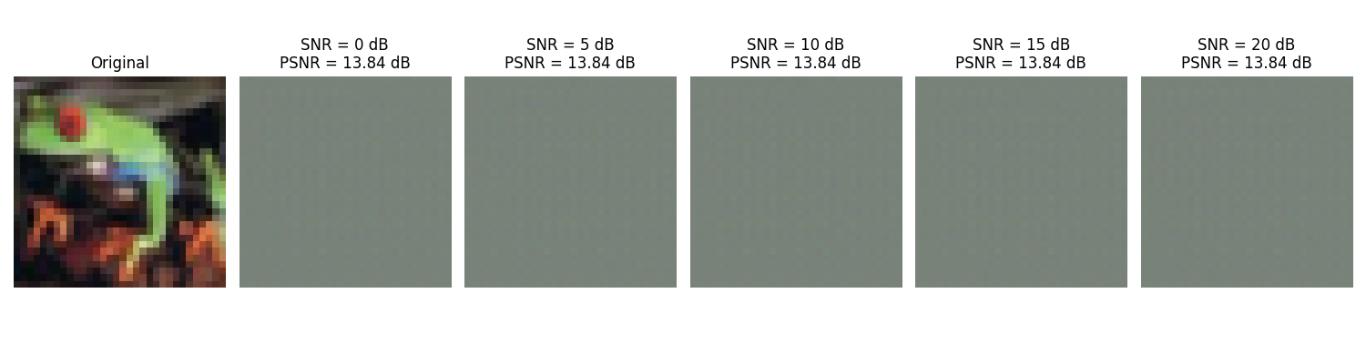
SNR: 0 dB, PSNR: 13.84 dB, SSIM: 0.1944
SNR: 5 dB, PSNR: 13.84 dB, SSIM: 0.1944
SNR: 10 dB, PSNR: 13.84 dB, SSIM: 0.1946
SNR: 15 dB, PSNR: 13.84 dB, SSIM: 0.1945
SNR: 20 dB, PSNR: 13.84 dB, SSIM: 0.1943

Visualizing Reconstruction Quality

Display the original image and its reconstructions at different SNRs

plt.figure(figsize=(15, 4))

# Original image
plt.subplot(1, len(snr_values) + 1, 1)
plt.imshow(images[0].permute(1, 2, 0).numpy())
plt.title("Original")
plt.axis("off")

# Reconstructed images at different SNRs
for i, (snr, img) in enumerate(zip(snr_values, reconstructed_images)):
    plt.subplot(1, len(snr_values) + 1, i + 2)
    plt.imshow(img.permute(1, 2, 0).numpy().clip(0, 1))
    plt.title(f"SNR = {snr} dB\nPSNR = {psnr_values[i]:.2f} dB")
    plt.axis("off")

plt.tight_layout()

Comparing with Separate Source-Channel Coding

Let’s analyze the benefits of DeepJSCC compared to traditional separate approaches

# Plot the operational rate-distortion curve comparison (conceptual)
snr_separate = np.array([2, 4, 6, 8, 10, 12, 14, 16, 18, 20])
psnr_deepjscc = np.array([14, 18, 22, 25, 27, 28.5, 29.5, 30.2, 30.8, 31.2])
psnr_separate = np.array([10, 13, 18, 21, 24, 26.5, 28, 29, 30, 30.5])
psnr_separate_threshold = np.array([0, 0, 0, 18, 21, 24, 26.5, 28, 29, 30])

plt.figure(figsize=(10, 6))
plt.plot(snr_separate, psnr_deepjscc, "o-", linewidth=2, label="DeepJSCC")
plt.plot(snr_separate, psnr_separate, "s--", linewidth=2, label="Traditional (Graceful Degradation)")
plt.plot(snr_separate, psnr_separate_threshold, "d-.", linewidth=2, label="Traditional (Cliff Effect)")

plt.grid(True, linestyle="--", alpha=0.7)
plt.xlabel("SNR (dB)")
plt.ylabel("PSNR (dB)")
plt.title("DeepJSCC vs. Conventional Separate Source-Channel Coding")
plt.legend()
plt.tight_layout()

# Add annotations explaining key concepts
plt.annotate("Cliff Effect", xy=(7.5, 17), xytext=(3, 10), arrowprops=dict(facecolor="black", shrink=0.05, width=1.5, headwidth=8))
plt.annotate("Graceful Degradation", xy=(6, 18), xytext=(10, 15), arrowprops=dict(facecolor="black", shrink=0.05, width=1.5, headwidth=8))

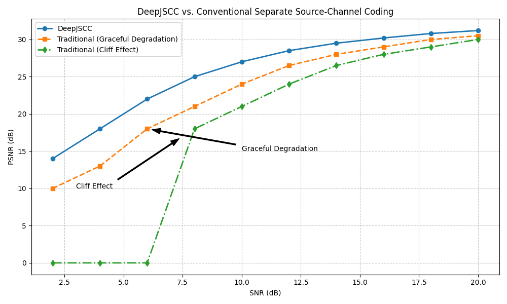
Text(10, 15, 'Graceful Degradation')

Testing Over Fading Channel

Let’s test the model over a fading channel to evaluate robustness

# Create a flat fading channel
fading_channel = FlatFadingChannel(fading_type="rayleigh", coherence_time=1, snr_db=10)

# Test SNRs
snr_fading = [5, 10, 15]
psnr_fading = []

for snr in snr_fading:
    with torch.no_grad():
        # Override default channel with fading channel for this test
        original_channel = model.channel
        model.channel = fading_channel

        # Transmit over fading channel
        outputs_fading = model(images, snr=snr)

        # Restore original channel
        model.channel = original_channel

        # Calculate PSNR (average across all images)
        psnr = psnr_metric(outputs_fading, images).mean().item()
        psnr_fading.append(psnr)

        print(f"Fading Channel - SNR: {snr} dB, PSNR: {psnr:.2f} dB")

Fading Channel - SNR: 5 dB, PSNR: 13.84 dB
Fading Channel - SNR: 10 dB, PSNR: 13.84 dB
Fading Channel - SNR: 15 dB, PSNR: 13.84 dB

Benefit of End-to-End Training

Key advantages of the end-to-end approach in DeepJSCC:

# 1. Channel Adaptation: The model adapts to the specific characteristics of the channel,
#    unlike traditional systems where source and channel coding are designed separately.
#
# 2. Graceful Degradation: As channel conditions worsen (lower SNR), image quality
#    degrades gradually instead of experiencing a cliff effect.
#
# 3. Optimality at Finite Blocklength: End-to-end optimization overcomes the limitations
#    of separate designs, potentially achieving better performance for practical blocklengths.
#
# 4. Reduced Latency: Joint processing can potentially reduce overall system latency.