LDPC Coding and Belief Propagation Decoding via RPTU Database

This example demonstrates Low-Density Parity-Check (LDPC) codes [Gallager, 1962] (via RPTU database) and belief propagation decoding [Kschischang et al., 2002]. We’ll simulate a complete communication system using LDPC codes over an AWGN channel and analyze the error performance at different SNR levels.

import matplotlib.pyplot as plt
import numpy as np
import seaborn as sns
import torch
from tqdm import tqdm

from kaira.channels.analog import AWGNChannel
from kaira.models.fec.decoders import BeliefPropagationDecoder
from kaira.models.fec.encoders import LDPCCodeEncoder
from kaira.modulations.psk import BPSKDemodulator, BPSKModulator
from kaira.utils import snr_to_noise_power

Setting up

First, we set a random seed to ensure reproducibility and configure our visualization settings.

torch.manual_seed(42)
np.random.seed(42)

# Configure better visualization settings
plt.style.use("seaborn-v0_8-whitegrid")
sns.set_context("notebook", font_scale=1.2)

LDPC Code Fundamentals

LDPC codes are defined by a sparse parity-check matrix H. Here we will use a LDPC code from RPTU code database with code_length = 672, code_dimension = 448.

# Define code parameters
code_length = 672  # Codeword length
code_dimension = 448  # Message length

device = torch.device("cuda" if torch.cuda.is_available() else "cpu")
# Load the parity-check matrix from the RPTU database
encoder = LDPCCodeEncoder(rptu_database=True, code_length=code_length, code_dimension=code_dimension, device=device)
# Print the parity-check matrix
parity_check_matrix = encoder.check_matrix.clone().cpu()

Loading LDPC code from RPTU database...
Michael Helmling, Stefan Scholl, Florian Gensheimer, Tobias Dietz, Kira Kraft, Oliver Griebel, Stefan Ruzika, and Norbert Wehn. Database of Channel Codes and ML Simulation Results. rptu.de/channel-codes, 2025.
------------------------------------
Using default rptu_standart='wimax' for (code_length=672, code_dimension=448).

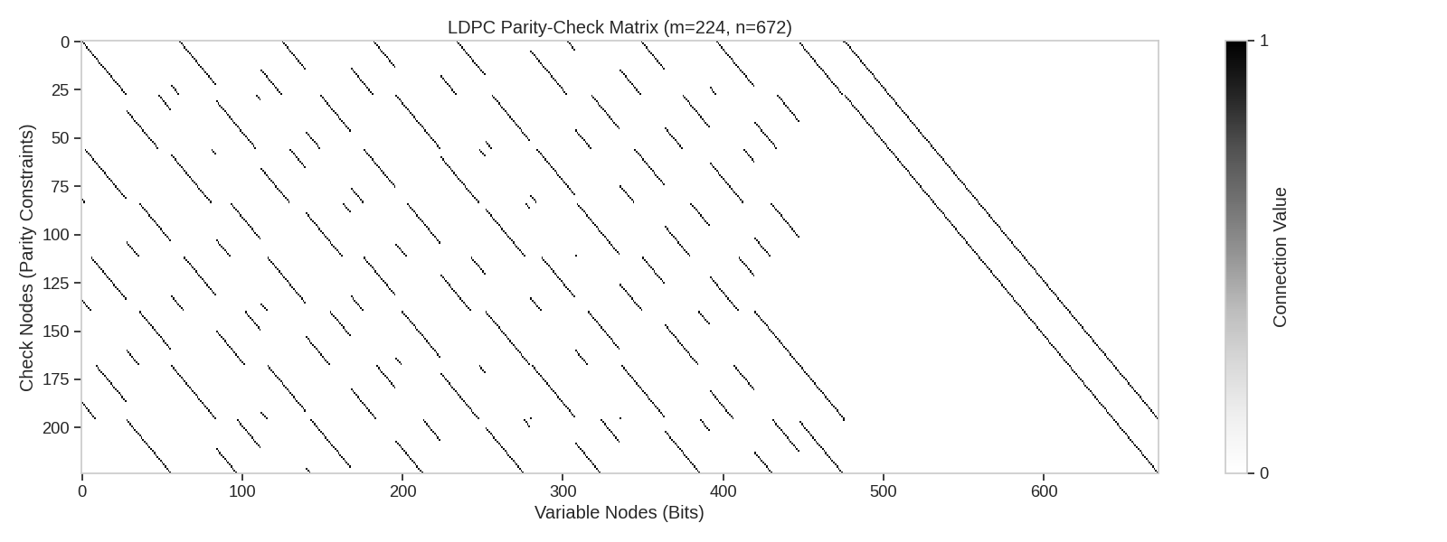
Visualizing the Parity-Check Matrix

We can visualize the parity-check matrix as a binary grid, which helps illustrate the sparsity pattern essential for LDPC codes.

plt.figure(figsize=(16, 6))
plt.imshow(parity_check_matrix, aspect="auto", cmap="Greys", interpolation="nearest")
plt.colorbar(ticks=[0, 1], label="Connection Value")
plt.xlabel("Variable Nodes (Bits)")
plt.ylabel("Check Nodes (Parity Constraints)")
plt.title(f"LDPC Parity-Check Matrix (m={parity_check_matrix.shape[0]}, n={parity_check_matrix.shape[1]})")
plt.grid(False)
plt.tight_layout()

Communication System Setup

We’ll set up a complete communication system with an LDPC encoder, an AWGN channel, and a belief propagation decoder.

# For LDPC codes, dimensions are determined from the parity check matrix
# The parity check matrix H has dimensions (n-k) x n, where:
# - n is the codeword length
# - k is the message length
# - (n-k) is the number of parity bits
parity_bits = parity_check_matrix.shape[0]
codeword_length = parity_check_matrix.shape[1]
message_length = codeword_length - parity_bits

print(f"Message length: {message_length} bits")
print(f"Codeword length: {codeword_length} bits")
print(f"Code rate: {message_length/codeword_length:.3f}")

Message length: 448 bits
Codeword length: 672 bits
Code rate: 0.667

Simulating Communication at Different SNR Levels

Let’s simulate the transmission of messages over an AWGN channel at various SNR levels and analyze the bit error rate performance.

snr_db_values = [-2, 0, 2, 4]
iterations_values = [5, 10, 20]
num_messages = 1000
batch_size = 100
results = {}

modulator = BPSKModulator(complex_output=False)
demodulator = BPSKDemodulator()


for bp_iters in iterations_values:
    ber_values = []
    bler_values = []

    # Initialize decoder with specific iteration count
    decoder = BeliefPropagationDecoder(encoder, bp_iters=bp_iters)

    for snr_db in tqdm(snr_db_values, desc=f"BP Iterations: {bp_iters}"):
        # Initialize the channel for current SNR
        noise_power = snr_to_noise_power(1.0, snr_db)
        channel = AWGNChannel(avg_noise_power=noise_power)

        # Counters for error statistics
        total_bits = 0
        error_bits = 0
        total_blocks = 0
        error_blocks = 0

        # Process messages in batches
        for i in range(0, num_messages, batch_size):
            # Generate random messages
            message = torch.randint(0, 2, (batch_size, message_length), dtype=torch.float32).to(device)

            # Encode the messages
            codeword = encoder(message)

            # Modulate the codewords to bipolar format
            bipolar_codeword = modulator(codeword)

            # Transmit over AWGN channel
            received_soft = channel(bipolar_codeword)

            # Demodulate the received signal
            demodulated_soft = demodulator(received_soft, noise_var=noise_power)

            # Decode the received signals
            decoded_message = decoder(demodulated_soft)

            # Calculate errors
            bit_errors = (message != decoded_message).to(torch.float32)
            block_errors = (torch.sum(bit_errors, dim=1) > 0).to(torch.float32)

            # Update statistics
            error_bits += torch.sum(bit_errors).item()
            total_bits += message.numel()
            error_blocks += torch.sum(block_errors).item()
            total_blocks += message.shape[0]

        # Calculate error rates
        ber = error_bits / total_bits
        bler = error_blocks / total_blocks

        ber_values.append(ber)
        bler_values.append(bler)

    results[bp_iters] = {"ber": ber_values, "bler": bler_values}

BP Iterations: 5:   0%|          | 0/4 [00:00<?, ?it/s]
BP Iterations: 5:  25%|██▌       | 1/4 [00:12<00:38, 12.81s/it]
BP Iterations: 5:  50%|█████     | 2/4 [00:25<00:25, 12.78s/it]
BP Iterations: 5:  75%|███████▌  | 3/4 [00:38<00:12, 12.73s/it]
BP Iterations: 5: 100%|██████████| 4/4 [00:50<00:00, 12.61s/it]
BP Iterations: 5: 100%|██████████| 4/4 [00:50<00:00, 12.67s/it]

BP Iterations: 10:   0%|          | 0/4 [00:00<?, ?it/s]
BP Iterations: 10:  25%|██▌       | 1/4 [00:25<01:16, 25.64s/it]
BP Iterations: 10:  50%|█████     | 2/4 [00:51<00:51, 25.63s/it]
BP Iterations: 10:  75%|███████▌  | 3/4 [01:16<00:25, 25.48s/it]
BP Iterations: 10: 100%|██████████| 4/4 [01:40<00:00, 25.03s/it]
BP Iterations: 10: 100%|██████████| 4/4 [01:40<00:00, 25.23s/it]

BP Iterations: 20:   0%|          | 0/4 [00:00<?, ?it/s]
BP Iterations: 20:  25%|██▌       | 1/4 [00:51<02:34, 51.54s/it]
BP Iterations: 20:  50%|█████     | 2/4 [01:42<01:42, 51.34s/it]
BP Iterations: 20:  75%|███████▌  | 3/4 [02:33<00:50, 50.94s/it]
BP Iterations: 20: 100%|██████████| 4/4 [03:20<00:00, 49.63s/it]
BP Iterations: 20: 100%|██████████| 4/4 [03:20<00:00, 50.21s/it]

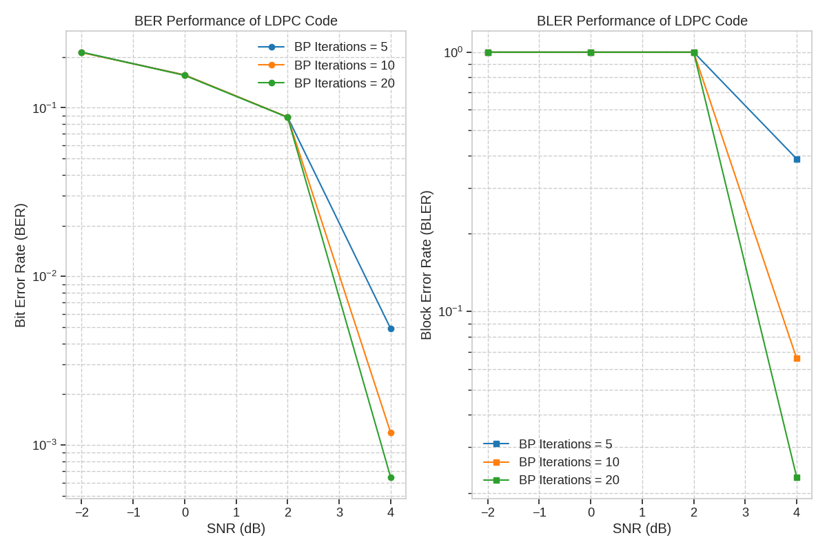
Performance Analysis

Let’s visualize the performance of our LDPC code with different numbers of belief propagation iterations across various SNR levels.

plt.figure(figsize=(12, 8))

# Plot Bit Error Rate
plt.subplot(1, 2, 1)
for bp_iters, data in results.items():
    plt.semilogy(snr_db_values, data["ber"], "o-", label=f"BP Iterations = {bp_iters}")
plt.grid(True, which="both", ls="--")
plt.xlabel("SNR (dB)")
plt.ylabel("Bit Error Rate (BER)")
plt.title("BER Performance of LDPC Code")
plt.legend()

# Plot Block Error Rate
plt.subplot(1, 2, 2)
for bp_iters, data in results.items():
    plt.semilogy(snr_db_values, data["bler"], "s-", label=f"BP Iterations = {bp_iters}")
plt.grid(True, which="both", ls="--")
plt.xlabel("SNR (dB)")
plt.ylabel("Block Error Rate (BLER)")
plt.title("BLER Performance of LDPC Code")
plt.legend()

plt.tight_layout()

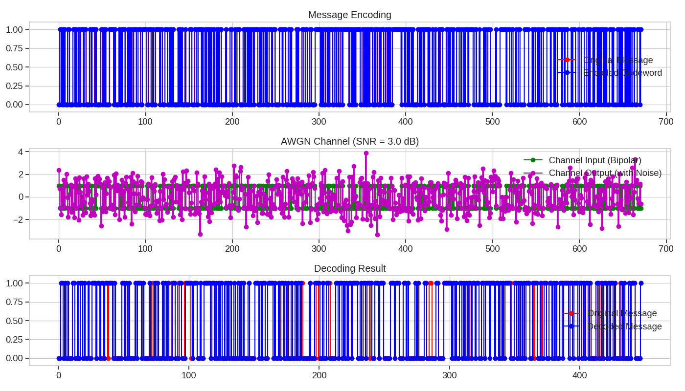
Single Message Example

Let’s walk through the encoding, transmission, and decoding process for a single message to better understand the flow.

# Generate a single random message
single_message = torch.randint(0, 2, (1, message_length), dtype=torch.float32).to(device)

# Encode the message
single_codeword = encoder(single_message)

# Set channel SNR
test_snr_db = 3.0
noise_power_test = snr_to_noise_power(1.0, test_snr_db)
test_channel = AWGNChannel(avg_noise_power=noise_power_test)

# Convert to bipolar format for AWGN channel
single_bipolar = modulator(single_codeword)

# Transmit over AWGN channel
single_received = test_channel(single_bipolar)

# Demodulate the received signal
single_demodulated = demodulator(single_received, noise_var=noise_power_test)

# Initialize decoder with 10 iterations
test_decoder = BeliefPropagationDecoder(encoder, bp_iters=10)

# Decode the received signal
single_decoded = test_decoder(single_demodulated)

# Check if successfully decoded
success = torch.all(single_message == single_decoded).item()

print(f"\nSingle Message Transmission Example (SNR = {test_snr_db} dB):")
print(f"Original message: {single_message.squeeze().int().tolist()}")
print(f"Encoded codeword: {single_codeword.squeeze().int().tolist()}")
print(f"Decoded message: {single_decoded.squeeze().int().tolist()}")
print(f"Decoding {'successful' if success else 'failed'}")

Single Message Transmission Example (SNR = 3.0 dB):
Original message: [0, 0, 1, 1, 0, 1, 0, 1, 0, 0, 0, 1, 1, 0, 0, 0, 0, 1, 1, 0, 1, 0, 0, 1, 0, 0, 1, 1, 1, 0, 1, 1, 0, 0, 0, 0, 1, 1, 0, 1, 1, 1, 0, 1, 0, 0, 0, 0, 0, 1, 1, 0, 1, 0, 1, 0, 0, 0, 0, 1, 1, 1, 1, 1, 0, 1, 0, 0, 0, 0, 1, 0, 1, 0, 1, 1, 1, 0, 0, 0, 1, 0, 1, 0, 1, 0, 0, 1, 1, 1, 0, 0, 1, 1, 1, 0, 0, 1, 1, 1, 1, 1, 0, 0, 1, 1, 1, 0, 0, 1, 0, 0, 1, 1, 1, 1, 1, 0, 1, 1, 0, 0, 0, 1, 1, 1, 0, 0, 1, 0, 1, 0, 1, 0, 0, 0, 0, 0, 1, 0, 1, 0, 1, 0, 0, 0, 1, 0, 0, 0, 0, 1, 1, 1, 0, 0, 0, 1, 1, 0, 0, 1, 1, 1, 1, 0, 1, 0, 0, 1, 0, 1, 1, 0, 1, 0, 1, 0, 0, 1, 0, 0, 1, 0, 1, 0, 1, 1, 0, 0, 0, 0, 0, 1, 0, 0, 0, 0, 1, 1, 0, 0, 0, 1, 0, 0, 1, 1, 1, 0, 0, 0, 0, 1, 1, 0, 1, 1, 0, 1, 0, 1, 0, 1, 1, 0, 1, 1, 1, 1, 0, 0, 1, 0, 1, 1, 0, 1, 1, 0, 1, 0, 0, 1, 1, 1, 0, 1, 1, 1, 0, 0, 0, 0, 0, 1, 1, 1, 0, 1, 1, 1, 0, 0, 0, 1, 1, 0, 1, 0, 0, 0, 0, 0, 1, 0, 1, 0, 0, 0, 0, 1, 1, 0, 0, 1, 1, 0, 0, 0, 1, 1, 0, 0, 0, 0, 1, 1, 1, 1, 1, 1, 0, 1, 0, 1, 0, 0, 1, 1, 0, 1, 0, 1, 1, 1, 0, 0, 1, 1, 0, 1, 1, 0, 0, 1, 1, 0, 1, 1, 1, 1, 1, 1, 1, 0, 1, 1, 0, 1, 0, 1, 0, 1, 1, 1, 1, 1, 0, 0, 1, 1, 0, 1, 0, 1, 0, 1, 0, 1, 1, 1, 0, 0, 1, 0, 1, 1, 0, 0, 1, 0, 1, 1, 1, 0, 0, 1, 1, 0, 1, 0, 1, 0, 0, 1, 1, 1, 1, 1, 1, 1, 1, 1, 1, 0, 1, 1, 1, 0, 1, 1, 0, 1, 0, 1, 1, 0, 1, 0, 0, 0, 0, 0, 1, 1, 0, 1, 0, 1, 1, 0, 1, 1, 1, 1, 0, 1, 0, 0, 0, 1, 0, 0, 1, 0, 0, 0, 1, 0, 1, 1, 1, 0, 0, 0, 0, 1]
Encoded codeword: [0, 0, 1, 1, 0, 1, 0, 1, 0, 0, 0, 1, 1, 0, 0, 0, 0, 1, 1, 0, 1, 0, 0, 1, 0, 0, 1, 1, 1, 0, 1, 1, 0, 0, 0, 0, 1, 1, 0, 1, 1, 1, 0, 1, 0, 0, 0, 0, 0, 1, 1, 0, 1, 0, 1, 0, 0, 0, 0, 1, 1, 1, 1, 1, 0, 1, 0, 0, 0, 0, 1, 0, 1, 0, 1, 1, 1, 0, 0, 0, 1, 0, 1, 0, 1, 0, 0, 1, 1, 1, 0, 0, 1, 1, 1, 0, 0, 1, 1, 1, 1, 1, 0, 0, 1, 1, 1, 0, 0, 1, 0, 0, 1, 1, 1, 1, 1, 0, 1, 1, 0, 0, 0, 1, 1, 1, 0, 0, 1, 0, 1, 0, 1, 0, 0, 0, 0, 0, 1, 0, 1, 0, 1, 0, 0, 0, 1, 0, 0, 0, 0, 1, 1, 1, 0, 0, 0, 1, 1, 0, 0, 1, 1, 1, 1, 0, 1, 0, 0, 1, 0, 1, 1, 0, 1, 0, 1, 0, 0, 1, 0, 0, 1, 0, 1, 0, 1, 1, 0, 0, 0, 0, 0, 1, 0, 0, 0, 0, 1, 1, 0, 0, 0, 1, 0, 0, 1, 1, 1, 0, 0, 0, 0, 1, 1, 0, 1, 1, 0, 1, 0, 1, 0, 1, 1, 0, 1, 1, 1, 1, 0, 0, 1, 0, 1, 1, 0, 1, 1, 0, 1, 0, 0, 1, 1, 1, 0, 1, 1, 1, 0, 0, 0, 0, 0, 1, 1, 1, 0, 1, 1, 1, 0, 0, 0, 1, 1, 0, 1, 0, 0, 0, 0, 0, 1, 0, 1, 0, 0, 0, 0, 1, 1, 0, 0, 1, 1, 0, 0, 0, 1, 1, 0, 0, 0, 0, 1, 1, 1, 1, 1, 1, 0, 1, 0, 1, 0, 0, 1, 1, 0, 1, 0, 1, 1, 1, 0, 0, 1, 1, 0, 1, 1, 0, 0, 1, 1, 0, 1, 1, 1, 1, 1, 1, 1, 0, 1, 1, 0, 1, 0, 1, 0, 1, 1, 1, 1, 1, 0, 0, 1, 1, 0, 1, 0, 1, 0, 1, 0, 1, 1, 1, 0, 0, 1, 0, 1, 1, 0, 0, 1, 0, 1, 1, 1, 0, 0, 1, 1, 0, 1, 0, 1, 0, 0, 1, 1, 1, 1, 1, 1, 1, 1, 1, 1, 0, 1, 1, 1, 0, 1, 1, 0, 1, 0, 1, 1, 0, 1, 0, 0, 0, 0, 0, 1, 1, 0, 1, 0, 1, 1, 0, 1, 1, 1, 1, 0, 1, 0, 0, 0, 1, 0, 0, 1, 0, 0, 0, 1, 0, 1, 1, 1, 0, 0, 0, 0, 1, 1, 0, 1, 0, 1, 1, 0, 1, 0, 0, 0, 1, 1, 1, 0, 0, 1, 0, 0, 1, 0, 1, 1, 1, 0, 1, 1, 1, 1, 1, 0, 0, 1, 1, 0, 0, 0, 1, 0, 0, 0, 0, 1, 0, 1, 0, 0, 1, 1, 1, 0, 0, 0, 0, 0, 0, 1, 0, 0, 0, 0, 1, 1, 1, 1, 1, 1, 1, 0, 1, 1, 1, 0, 0, 1, 1, 0, 0, 0, 1, 0, 0, 1, 1, 0, 0, 0, 0, 0, 1, 1, 1, 1, 1, 0, 0, 0, 0, 1, 0, 1, 1, 0, 0, 1, 0, 1, 0, 0, 1, 1, 0, 0, 0, 0, 1, 1, 1, 1, 0, 1, 1, 1, 0, 1, 0, 0, 1, 1, 1, 1, 1, 0, 1, 1, 0, 1, 1, 1, 0, 0, 0, 0, 1, 0, 1, 1, 1, 0, 0, 0, 1, 1, 0, 0, 1, 1, 1, 0, 0, 0, 1, 1, 0, 1, 0, 0, 0, 1, 0, 1, 1, 1, 0, 1, 0, 1, 0, 1, 1, 0, 1, 0, 1, 0, 0, 0, 1, 1, 1, 0, 1, 0, 0, 0, 0, 1, 1, 0, 1, 0, 1, 0, 0, 0, 1, 0, 1, 0, 1, 0, 1, 0, 0, 1, 1, 0, 0, 0, 1, 1, 1, 0, 1]
Decoded message: [0, 0, 1, 1, 0, 1, 0, 1, 0, 0, 0, 1, 1, 0, 0, 1, 0, 1, 1, 0, 1, 0, 0, 1, 0, 0, 1, 1, 1, 0, 1, 1, 0, 1, 1, 0, 1, 1, 1, 1, 1, 1, 0, 1, 0, 0, 0, 0, 0, 1, 1, 0, 1, 0, 1, 0, 0, 0, 0, 1, 0, 1, 1, 1, 0, 1, 0, 0, 0, 0, 1, 0, 0, 0, 1, 0, 1, 0, 0, 0, 1, 0, 1, 0, 1, 0, 0, 0, 1, 1, 0, 0, 0, 1, 1, 0, 0, 0, 1, 1, 1, 1, 1, 0, 1, 1, 1, 0, 0, 1, 0, 0, 1, 1, 1, 1, 1, 0, 1, 1, 0, 1, 0, 1, 0, 1, 0, 0, 1, 0, 1, 0, 1, 0, 0, 1, 0, 0, 1, 0, 1, 0, 1, 0, 0, 0, 1, 0, 0, 0, 0, 1, 1, 1, 0, 1, 0, 1, 1, 0, 0, 1, 1, 1, 1, 0, 1, 0, 0, 1, 0, 1, 1, 0, 1, 0, 1, 0, 0, 1, 0, 0, 1, 0, 1, 0, 1, 0, 0, 0, 0, 0, 0, 1, 0, 0, 0, 1, 1, 1, 1, 0, 0, 1, 0, 0, 1, 1, 0, 0, 0, 0, 0, 1, 1, 0, 1, 1, 0, 1, 0, 1, 0, 1, 1, 0, 1, 1, 1, 1, 0, 0, 1, 0, 1, 1, 0, 1, 1, 1, 1, 0, 0, 1, 1, 1, 0, 1, 1, 1, 0, 0, 0, 0, 0, 1, 1, 1, 0, 1, 1, 1, 0, 0, 0, 1, 1, 0, 1, 0, 0, 0, 0, 0, 1, 0, 1, 0, 0, 0, 0, 1, 1, 0, 0, 0, 0, 0, 0, 0, 1, 1, 0, 0, 0, 0, 1, 1, 1, 1, 1, 1, 0, 1, 0, 1, 0, 0, 1, 1, 0, 1, 0, 1, 0, 1, 1, 0, 1, 1, 0, 1, 1, 0, 0, 1, 1, 0, 1, 1, 1, 0, 1, 1, 1, 0, 1, 1, 0, 1, 0, 1, 0, 1, 1, 1, 1, 0, 0, 0, 1, 1, 0, 1, 0, 1, 0, 1, 0, 1, 1, 1, 0, 0, 1, 1, 1, 1, 0, 0, 1, 0, 0, 1, 1, 0, 0, 1, 1, 0, 1, 0, 1, 0, 0, 1, 1, 0, 1, 1, 1, 1, 0, 1, 1, 0, 1, 1, 1, 0, 1, 1, 0, 1, 0, 1, 1, 0, 1, 0, 0, 0, 0, 1, 1, 0, 0, 1, 0, 1, 1, 0, 1, 0, 1, 1, 0, 1, 0, 0, 0, 0, 1, 0, 1, 0, 0, 0, 1, 0, 1, 1, 1, 0, 0, 0, 0, 1]
Decoding failed

Visualizing the Transmission Process

Let’s visualize the transmission process for our single message example.

single_message = single_message.clone().cpu()
single_codeword = single_codeword.clone().cpu()
single_bipolar = single_bipolar.clone().cpu()
single_received = single_received.clone().cpu()
single_decoded = single_decoded.clone().cpu()

plt.figure(figsize=(14, 8))

# Plot original and encoded messages
plt.subplot(3, 1, 1)
plt.step(range(message_length), single_message.squeeze(), "ro-", where="mid", label="Original Message")
plt.step(range(codeword_length), single_codeword.squeeze(), "bo-", where="mid", label="Encoded Codeword")
plt.grid(True)
plt.legend()
plt.title("Message Encoding")
plt.ylim(-0.1, 1.1)

# Plot channel input and output
plt.subplot(3, 1, 2)
plt.step(range(codeword_length), single_bipolar.squeeze(), "go-", where="mid", label="Channel Input (Bipolar)")
plt.step(range(codeword_length), single_received.squeeze(), "mo-", where="mid", label="Channel Output (with Noise)")
plt.grid(True)
plt.legend()
plt.title(f"AWGN Channel (SNR = {test_snr_db} dB)")

# Plot comparison of original and decoded messages
plt.subplot(3, 1, 3)
plt.step(range(message_length), single_message.squeeze(), "ro-", where="mid", label="Original Message")
plt.step(range(message_length), single_decoded.squeeze(), "bo-", where="mid", label="Decoded Message")
plt.grid(True)
plt.legend()
plt.title("Decoding Result")
plt.ylim(-0.1, 1.1)

plt.tight_layout()
plt.show()

Conclusion

This example demonstrates how LDPC codes [Gallager, 1962] can effectively correct errors introduced by noisy channels. We’ve shown how the performance improves with increased SNR and more decoding iterations.

LDPC codes are widely used in modern communication systems due to their excellent error-correcting capabilities that approach the Shannon limit. The belief propagation algorithm [Kschischang et al., 2002] provides an efficient decoding method that works well for sparse parity-check matrices.