Polar Coding and Decoding: Successive Cancellation and Belief Propagation

This example demonstrates Polar codes [Arıkan, 2008] with successive cancellation [Arıkan, 2009] and belief propagation decoding [Arıkan, 2011]. We’ll simulate a complete communication system using Polar codes over an AWGN channel and analyze the error performance at different SNR levels.

import matplotlib.pyplot as plt
import numpy as np
import seaborn as sns
import torch
from tqdm import tqdm

from kaira.channels.analog import AWGNChannel
from kaira.models.fec.decoders import BeliefPropagationPolarDecoder, SuccessiveCancellationDecoder
from kaira.models.fec.encoders import PolarCodeEncoder
from kaira.modulations.psk import BPSKDemodulator, BPSKModulator
from kaira.utils import snr_to_noise_power

Setting up

First, we set a random seed to ensure reproducibility and configure our visualization settings.

torch.manual_seed(42)
np.random.seed(42)

# Configure better visualization settings
plt.style.use("seaborn-v0_8-whitegrid")
sns.set_context("notebook", font_scale=1.2)

Polar Code Fundamentals

Polar codes are defined by a polar transformation Here we will use a Polar code with code_length = 32.

# Define code parameters
code_length = 32  # Codeword length
code_dimension = 32  # Message length

device = torch.device("cuda" if torch.cuda.is_available() else "cpu")
# Load the polar code encoder with the specified rank as in 5G standard.
encoder = PolarCodeEncoder(code_dimension=code_dimension, code_length=code_length, device=device, polar_i=False, load_rank=True, frozen_zeros=False)
generator_matrix = encoder.get_generator_matrix()

Loading rank polar indices as defined in 5G standard...

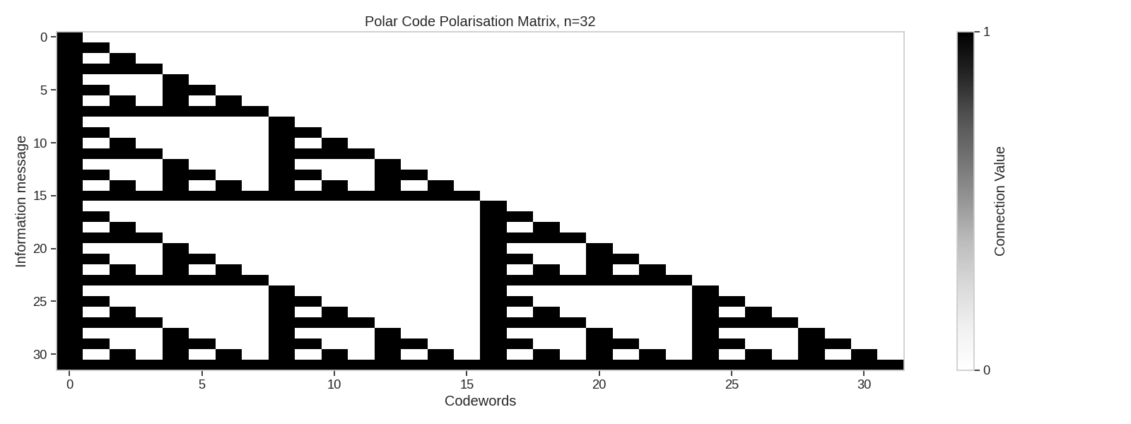
Visualizing the Generator Matrix

We can visualize the generator (polarization) matrix as a binary grid, which helps illustrate the polarization process.

plt.figure(figsize=(16, 6))
plt.imshow(generator_matrix.cpu().numpy(), aspect="auto", cmap="Greys", interpolation="nearest")
plt.colorbar(ticks=[0, 1], label="Connection Value")
plt.xlabel("Codewords")
plt.ylabel("Information message")
plt.title(f"Polar Code Polarisation Matrix, n={code_length}")
plt.grid(False)
plt.tight_layout()

Communication System Setup

We’ll set up a complete communication system with an Polar code encoder, an AWGN channel, and a belief propagation and a successive cancellation decoders.

# For polar codes, the code length should be # a power of 2,
# and the message length should be less than the code length.:
code_dimension = 64  # Codeword length
code_length = 128  # Message length

print(f"Message length: {code_dimension} bits")
print(f"Codeword length: {code_length} bits")
print(f"Code rate: {code_dimension/code_length:.3f}")

encoder = PolarCodeEncoder(code_dimension=code_dimension, code_length=code_length, device=device, polar_i=False, load_rank=True, frozen_zeros=False)

decoder_sc = SuccessiveCancellationDecoder(encoder, regime="sum_product")

decoders_arr = [decoder_sc]
decoders_names = ["SC"]
iterations_values = [5, 10, 20, 35]
for bp_iters in iterations_values:
    decoder_bp = BeliefPropagationPolarDecoder(encoder, bp_iters=bp_iters, early_stop=True, regime="sum_product", perm=None)
    decoders_arr.append(decoder_bp)
    decoders_names.append(f"BP Iter.: {bp_iters}")

decoder_bp = BeliefPropagationPolarDecoder(encoder, bp_iters=5, early_stop=True, regime="sum_product", perm="cycle")
decoders_arr.append(decoder_bp)
decoders_names.append(f"BP Iter.: {5} and cycle perm.")


# # %%
# # Simulating Communication at Different SNR Levels
# # --------------------------------------------------------------------------------------
# # Let's simulate the transmission of messages over an AWGN channel at various
# # SNR levels and analyze the bit error rate performance of different decoders.

snr_db_values = [-2, 0, 2, 4]
num_messages = 100000
batch_size = 1000
results = {}

modulator = BPSKModulator(complex_output=False)
demodulator = BPSKDemodulator()


for i, decoder in enumerate(decoders_arr):
    ber_values = []
    bler_values = []

    # Initialize decoder with specific iteration count
    decoder = decoder.to(device)

    for snr_db in tqdm(snr_db_values, desc=decoders_names[i]):
        # Initialize the channel for current SNR
        noise_power = snr_to_noise_power(1.0, snr_db)
        channel = AWGNChannel(avg_noise_power=noise_power)

        # Counters for error statistics
        total_bits = 0
        error_bits = 0
        total_blocks = 0
        error_blocks = 0

        # Process messages in batches
        for j in range(0, num_messages, batch_size):
            # Generate random messages
            message = torch.randint(0, 2, (batch_size, code_dimension), dtype=torch.float32).to(device)

            # Encode the messages
            codeword = encoder(message)

            # Modulate the codewords to bipolar format
            bipolar_codeword = modulator(codeword)

            # Transmit over AWGN channel
            received_soft = channel(bipolar_codeword)

            # Demodulate the received signal
            demodulated_soft = demodulator(received_soft, noise_var=noise_power)

            # Decode the received signals
            decoded_message = decoder(demodulated_soft)

            # Calculate errors
            bit_errors = (message != decoded_message).to(torch.float32)
            block_errors = (torch.sum(bit_errors, dim=1) > 0).to(torch.float32)

            # Update statistics
            error_bits += torch.sum(bit_errors).item()
            total_bits += message.numel()
            error_blocks += torch.sum(block_errors).item()
            total_blocks += message.shape[0]

        # Calculate error rates
        ber = error_bits / total_bits
        bler = error_blocks / total_blocks

        ber_values.append(ber)
        bler_values.append(bler)

    results[decoders_names[i]] = {"ber": ber_values, "bler": bler_values}

Message length: 64 bits
Codeword length: 128 bits
Code rate: 0.500
Loading rank polar indices as defined in 5G standard...
Decoder type: BeliefPropagationPolarDecoder, Polar Code Length: 128, Polar Code Dimension: 64, Number of iterations: 5, Function used during decoding: sum_product, Early Stop: True, Permutations: None
Decoder type: BeliefPropagationPolarDecoder, Polar Code Length: 128, Polar Code Dimension: 64, Number of iterations: 10, Function used during decoding: sum_product, Early Stop: True, Permutations: None
Decoder type: BeliefPropagationPolarDecoder, Polar Code Length: 128, Polar Code Dimension: 64, Number of iterations: 20, Function used during decoding: sum_product, Early Stop: True, Permutations: None
Decoder type: BeliefPropagationPolarDecoder, Polar Code Length: 128, Polar Code Dimension: 64, Number of iterations: 35, Function used during decoding: sum_product, Early Stop: True, Permutations: None
Decoder type: BeliefPropagationPolarDecoder, Polar Code Length: 128, Polar Code Dimension: 64, Number of iterations: 5, Function used during decoding: sum_product, Early Stop: True, Permutations: cycle

SC:   0%|          | 0/4 [00:00<?, ?it/s]
SC:  25%|██▌       | 1/4 [00:03<00:10,  3.36s/it]
SC:  50%|█████     | 2/4 [00:06<00:06,  3.39s/it]
SC:  75%|███████▌  | 3/4 [00:10<00:03,  3.38s/it]
SC: 100%|██████████| 4/4 [00:13<00:00,  3.37s/it]
SC: 100%|██████████| 4/4 [00:13<00:00,  3.37s/it]

BP Iter.: 5:   0%|          | 0/4 [00:00<?, ?it/s]
BP Iter.: 5:  25%|██▌       | 1/4 [00:15<00:46, 15.63s/it]
BP Iter.: 5:  50%|█████     | 2/4 [00:30<00:30, 15.31s/it]
BP Iter.: 5:  75%|███████▌  | 3/4 [00:43<00:14, 14.30s/it]
BP Iter.: 5: 100%|██████████| 4/4 [00:53<00:00, 12.36s/it]
BP Iter.: 5: 100%|██████████| 4/4 [00:53<00:00, 13.30s/it]

BP Iter.: 10:   0%|          | 0/4 [00:00<?, ?it/s]
BP Iter.: 10:  25%|██▌       | 1/4 [00:31<01:34, 31.34s/it]
BP Iter.: 10:  50%|█████     | 2/4 [00:59<00:59, 29.64s/it]
BP Iter.: 10:  75%|███████▌  | 3/4 [01:17<00:24, 24.25s/it]
BP Iter.: 10: 100%|██████████| 4/4 [01:28<00:00, 19.12s/it]
BP Iter.: 10: 100%|██████████| 4/4 [01:28<00:00, 22.22s/it]

BP Iter.: 20:   0%|          | 0/4 [00:00<?, ?it/s]
BP Iter.: 20:  25%|██▌       | 1/4 [01:00<03:00, 60.27s/it]
BP Iter.: 20:  50%|█████     | 2/4 [01:53<01:51, 55.91s/it]
BP Iter.: 20:  75%|███████▌  | 3/4 [02:18<00:41, 41.94s/it]
BP Iter.: 20: 100%|██████████| 4/4 [02:32<00:00, 31.01s/it]
BP Iter.: 20: 100%|██████████| 4/4 [02:32<00:00, 38.18s/it]

BP Iter.: 35:   0%|          | 0/4 [00:00<?, ?it/s]
BP Iter.: 35:  25%|██▌       | 1/4 [01:45<05:16, 105.54s/it]
BP Iter.: 35:  50%|█████     | 2/4 [03:15<03:12, 96.13s/it]
BP Iter.: 35:  75%|███████▌  | 3/4 [03:51<01:08, 68.64s/it]
BP Iter.: 35: 100%|██████████| 4/4 [04:09<00:00, 48.75s/it]
BP Iter.: 35: 100%|██████████| 4/4 [04:09<00:00, 62.32s/it]

BP Iter.: 5 and cycle perm.:   0%|          | 0/4 [00:00<?, ?it/s]
BP Iter.: 5 and cycle perm.:  25%|██▌       | 1/4 [01:43<05:11, 103.85s/it]
BP Iter.: 5 and cycle perm.:  50%|█████     | 2/4 [03:23<03:22, 101.18s/it]
BP Iter.: 5 and cycle perm.:  75%|███████▌  | 3/4 [04:11<01:17, 77.03s/it]
BP Iter.: 5 and cycle perm.: 100%|██████████| 4/4 [04:33<00:00, 55.30s/it]
BP Iter.: 5 and cycle perm.: 100%|██████████| 4/4 [04:33<00:00, 68.36s/it]

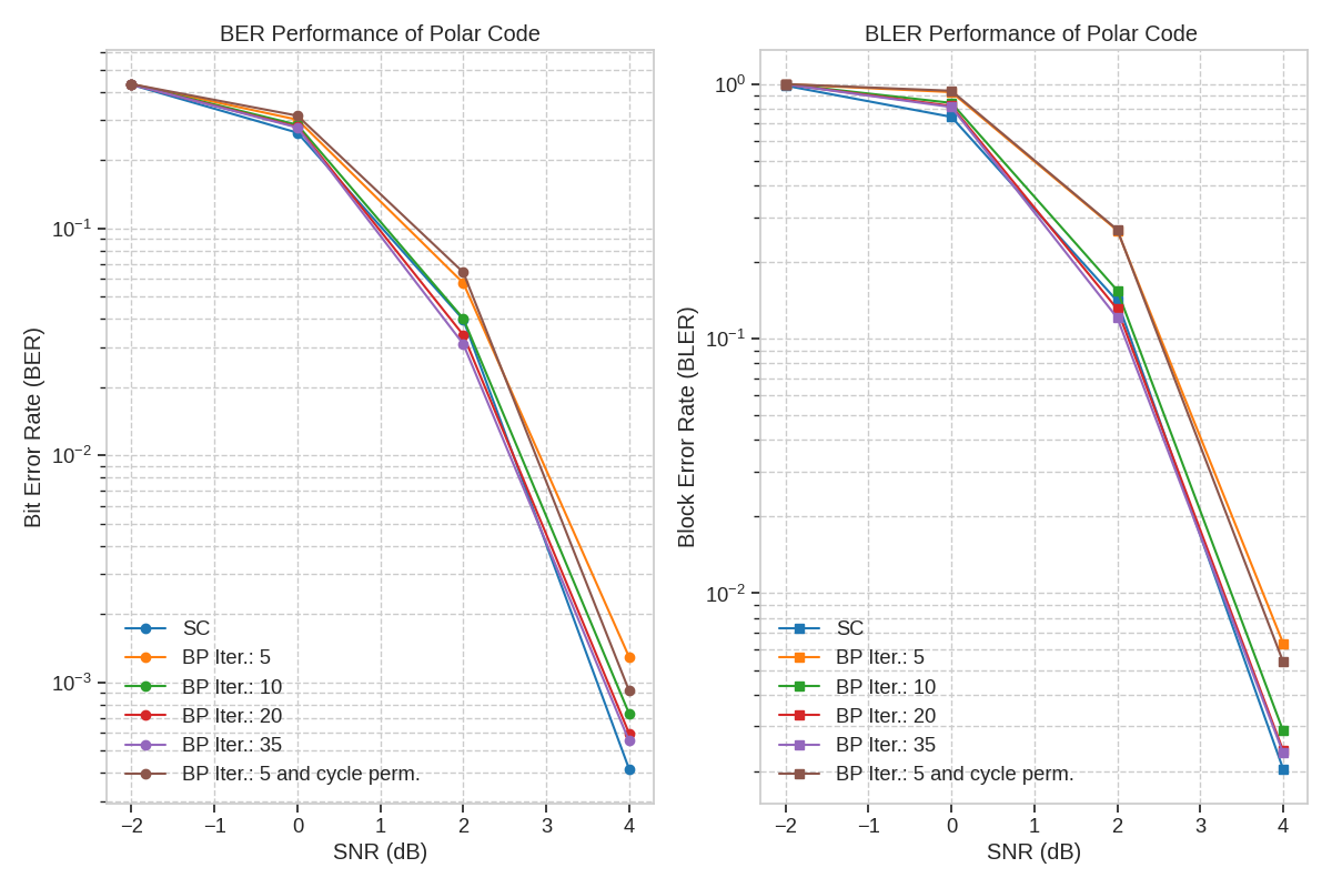
Performance Analysis

Let’s visualize the performance of our Polar code with different decoders across various SNR levels.

plt.figure(figsize=(12, 8))

# Plot Bit Error Rate
plt.subplot(1, 2, 1)
i = 0
for name, data in results.items():
    plt.semilogy(snr_db_values, data["ber"], "o-", label=name)
    i += 1
plt.grid(True, which="both", ls="--")
plt.xlabel("SNR (dB)")
plt.ylabel("Bit Error Rate (BER)")
plt.title("BER Performance of Polar Code")
plt.legend()

# Plot Block Error Rate
plt.subplot(1, 2, 2)
i = 0
for name, data in results.items():
    plt.semilogy(snr_db_values, data["bler"], "s-", label=name)
    i += 1
plt.grid(True, which="both", ls="--")
plt.xlabel("SNR (dB)")
plt.ylabel("Block Error Rate (BLER)")
plt.title("BLER Performance of Polar Code ")
plt.legend()

plt.tight_layout()

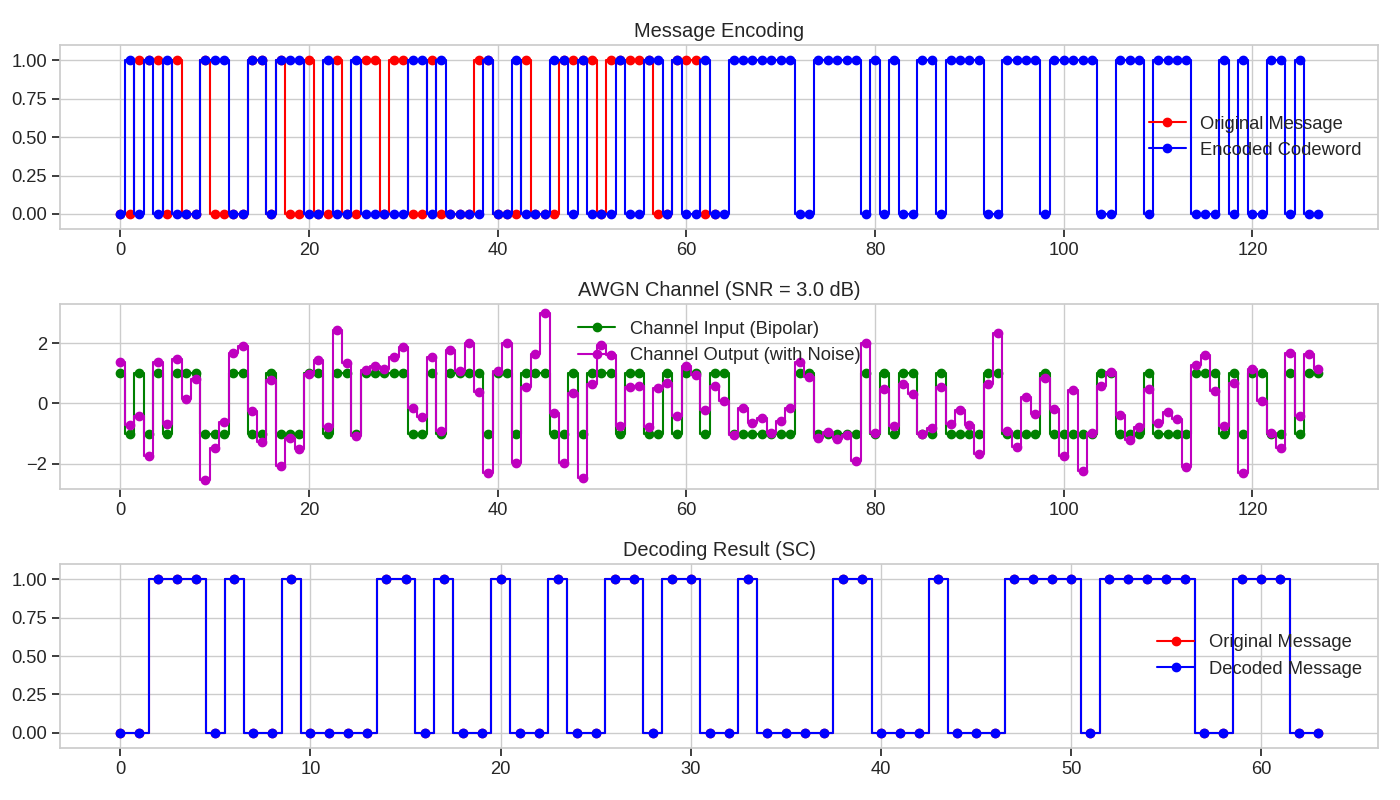
Single Message Example

Let’s walk through the encoding, transmission, and decoding process for a single message to better understand the flow.

# Generate a single random message
single_message = torch.randint(0, 2, (1, code_dimension), dtype=torch.float32).to(device)

# Encode the message
single_codeword = encoder(single_message)

# Set channel SNR
test_snr_db = 3.0
noise_power_test = snr_to_noise_power(1.0, test_snr_db)
test_channel = AWGNChannel(avg_noise_power=noise_power_test)

# Convert to bipolar format for AWGN channel
single_bipolar = modulator(single_codeword)

# Transmit over AWGN channel
single_received = test_channel(single_bipolar)

# Demodulate the received signal
single_demodulated = demodulator(single_received, noise_var=noise_power_test)

# Initialize Successive Cancellation Decoder
test_decoder = SuccessiveCancellationDecoder(encoder, regime="sum_product")

# Decode the received signal
single_decoded = test_decoder(single_demodulated)

# Check if successfully decoded
success = torch.all(single_message == single_decoded).item()

print(f"\nSingle Message Transmission Example (SNR = {test_snr_db} dB):")
print(f"Original message: {single_message.squeeze().int().tolist()}")
print(f"Encoded codeword: {single_codeword.squeeze().int().tolist()}")
print(f"Decoded message: {single_decoded.squeeze().int().tolist()}")
print(f"Decoding {'successful' if success else 'failed'}")

Single Message Transmission Example (SNR = 3.0 dB):
Original message: [0, 0, 1, 1, 1, 0, 1, 0, 0, 1, 0, 0, 0, 0, 1, 1, 0, 1, 0, 0, 1, 0, 0, 1, 0, 0, 1, 1, 0, 1, 1, 0, 0, 1, 0, 0, 0, 0, 1, 1, 0, 0, 0, 1, 0, 0, 0, 1, 1, 1, 1, 0, 1, 1, 1, 1, 1, 0, 0, 1, 1, 1, 0, 0]
Encoded codeword: [0, 1, 0, 1, 0, 1, 0, 0, 0, 1, 1, 1, 0, 0, 1, 1, 0, 1, 1, 1, 0, 0, 1, 0, 0, 1, 0, 0, 0, 0, 0, 1, 1, 0, 1, 0, 0, 0, 0, 1, 0, 0, 1, 0, 0, 0, 1, 1, 0, 1, 0, 0, 0, 1, 0, 0, 1, 1, 0, 1, 0, 0, 1, 0, 0, 1, 1, 1, 1, 1, 1, 1, 0, 0, 1, 1, 1, 1, 1, 0, 1, 0, 1, 0, 0, 1, 1, 0, 1, 1, 1, 1, 0, 0, 1, 1, 1, 1, 0, 1, 1, 1, 1, 1, 0, 0, 1, 1, 1, 0, 1, 1, 1, 1, 0, 0, 0, 1, 0, 1, 0, 0, 1, 1, 0, 1, 0, 0]
Decoded message: [0, 0, 1, 1, 1, 0, 1, 0, 0, 1, 0, 0, 0, 0, 1, 1, 0, 1, 0, 0, 1, 0, 0, 1, 0, 0, 1, 1, 0, 1, 1, 0, 0, 1, 0, 0, 0, 0, 1, 1, 0, 0, 0, 1, 0, 0, 0, 1, 1, 1, 1, 0, 1, 1, 1, 1, 1, 0, 0, 1, 1, 1, 0, 0]
Decoding successful

Visualizing the Transmission Process

Let’s visualize the transmission process for our single message example.

single_message = single_message.clone().cpu()
single_codeword = single_codeword.clone().cpu()
single_bipolar = single_bipolar.clone().cpu()
single_received = single_received.clone().cpu()
single_decoded = single_decoded.clone().cpu()

plt.figure(figsize=(14, 8))

# Plot original and encoded messages
plt.subplot(3, 1, 1)
plt.step(range(code_dimension), single_message.squeeze(), "ro-", where="mid", label="Original Message")
plt.step(range(code_length), single_codeword.squeeze(), "bo-", where="mid", label="Encoded Codeword")
plt.grid(True)
plt.legend()
plt.title("Message Encoding")
plt.ylim(-0.1, 1.1)

# Plot channel input and output
plt.subplot(3, 1, 2)
plt.step(range(code_length), single_bipolar.squeeze(), "go-", where="mid", label="Channel Input (Bipolar)")
plt.step(range(code_length), single_received.squeeze(), "mo-", where="mid", label="Channel Output (with Noise)")
plt.grid(True)
plt.legend()
plt.title(f"AWGN Channel (SNR = {test_snr_db} dB)")

# Plot comparison of original and decoded messages
plt.subplot(3, 1, 3)
plt.step(range(code_dimension), single_message.squeeze(), "ro-", where="mid", label="Original Message")
plt.step(range(code_dimension), single_decoded.squeeze(), "bo-", where="mid", label="Decoded Message")
plt.grid(True)
plt.legend()
plt.title("Decoding Result (SC)")
plt.ylim(-0.1, 1.1)

plt.tight_layout()
plt.show()

Conclusion

This example demonstrates how Polar codes [Arıkan, 2008] can effectively correct errors introduced by noisy channels. We’ve shown how the performance improves with increased SNR and more different decoding configurations.

Polar codes are widely used in modern communication systems due to their excellent error-correcting capabilities that approach the Shannon limit. The successive cancellation [Arıkan, 2009] and belief propagation algorithms [Arıkan, 2011] provides an efficient decoding for polar codes.