Modulation Schemes Comparison

This example provides a comprehensive comparison of different digital modulation schemes available in Kaira, including PSK, QAM, and PAM. We’ll analyze their constellation diagrams, spectral efficiency, and bit error rate performance.

import matplotlib.pyplot as plt

Imports and Setup

import numpy as np
import torch

from kaira.channels import AWGNChannel
from kaira.metrics.signal import BER
from kaira.modulations import (
    BPSKDemodulator,
    BPSKModulator,
    PAMDemodulator,
    PAMModulator,
    QAMDemodulator,
    QAMModulator,
    QPSKDemodulator,
    QPSKModulator,
)
from kaira.modulations.utils import plot_constellation
from kaira.utils import snr_to_noise_power

# Set random seed for reproducibility
torch.manual_seed(42)
np.random.seed(42)

Create Different Modulators and Demodulators

n_symbols = 1000

# Create modulators and demodulators
modulators = {
    "BPSK": (BPSKModulator(), BPSKDemodulator()),
    "QPSK": (QPSKModulator(), QPSKDemodulator()),
    "16-QAM": (QAMModulator(order=16), QAMDemodulator(order=16)),
    "64-QAM": (QAMModulator(order=64), QAMDemodulator(order=64)),
    "PAM-4": (PAMModulator(order=4), PAMDemodulator(order=4)),
    "PAM-8": (PAMModulator(order=8), PAMDemodulator(order=8)),
}

# Calculate bits per symbol for each scheme
bits_per_symbol = {"BPSK": 1, "QPSK": 2, "16-QAM": 4, "64-QAM": 6, "PAM-4": 2, "PAM-8": 3}

# Generate and modulate random bits for each scheme
input_bits = {}
modulated_symbols = {}
for name, (modulator, _) in modulators.items():
    n_bits = bits_per_symbol[name] * n_symbols
    input_bits[name] = torch.randint(0, 2, (1, n_bits))
    modulated_symbols[name] = modulator(input_bits[name])

Plot Constellation Diagrams

fig, axes = plt.subplots(2, 3, figsize=(15, 10))
for i, (name, symbols) in enumerate(modulated_symbols.items()):
    # Calculate row and column position
    row, col = divmod(i, 3)
    ax = axes[row, col]
    plot_constellation(symbols.flatten(), title=f"{name} Constellation", marker=".", ax=ax)
    ax.grid(True)
plt.tight_layout()
plt.show()

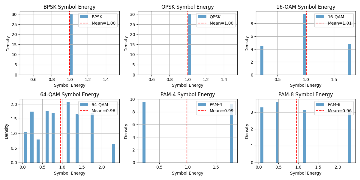
Compare Symbol Energy Distribution

fig, axes = plt.subplots(2, 3, figsize=(12, 6))
# Plot symbol energy distribution
for i, (name, symbols) in enumerate(modulated_symbols.items()):
    # Calculate row and column position
    row, col = divmod(i, 3)
    ax = axes[row, col]
    # Use .real to explicitly take only the real part for the histogram
    energy = torch.abs(symbols) ** 2
    energy_real = energy.real if torch.is_complex(energy) else energy
    ax.hist(energy_real.numpy().flatten(), bins=30, density=True, alpha=0.7, label=name)
    ax.set_title(f"{name} Symbol Energy")
    ax.set_xlabel("Symbol Energy")
    ax.set_ylabel("Density")
    ax.grid(True)
    # Add mean energy line
    mean_energy = torch.mean(energy_real).item()
    ax.axvline(mean_energy, color="r", linestyle="--", label=f"Mean={mean_energy:.2f}")
    ax.legend()
plt.tight_layout()
plt.show()

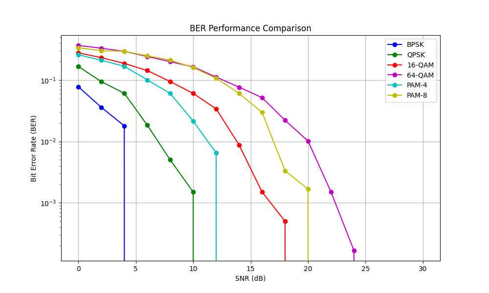
Compare BER Performance

snr_db_range = np.arange(0, 31, 2)
ber_results: dict[str, list[float]] = {name: [] for name in modulators.keys()}

# Initialize BER metric
ber_metric = BER()

for snr_db in snr_db_range:
    noise_power = snr_to_noise_power(1.0, snr_db)
    channel = AWGNChannel(avg_noise_power=noise_power)

    for name, (modulator, demodulator) in modulators.items():
        # Transmit through channel
        received = channel(modulated_symbols[name])

        # Demodulate using the corresponding demodulator
        demod_bits = demodulator(received)

        # Calculate BER
        ber = ber_metric(demod_bits, input_bits[name]).item()
        ber_results[name].append(ber)

# Plot BER curves
plt.figure(figsize=(10, 6))
colors = ["b", "g", "r", "m", "c", "y"]

for (name, ber), color in zip(ber_results.items(), colors):
    plt.semilogy(snr_db_range, ber, f"{color}o-", label=name)

plt.grid(True)
plt.xlabel("SNR (dB)")
plt.ylabel("Bit Error Rate (BER)")
plt.title("BER Performance Comparison")
plt.legend()
plt.show()

Compare Spectral Efficiency and Power Requirements

plt.figure(figsize=(12, 5))

# Create subplots
ax1 = plt.subplot(121)
ax2 = plt.subplot(122)

# Plot spectral efficiency
schemes = list(modulators.keys())
efficiency = [bits_per_symbol[name] for name in schemes]

ax1.bar(schemes, efficiency)
ax1.set_ylabel("Spectral Efficiency (bits/symbol)")
ax1.set_title("Spectral Efficiency Comparison")
plt.setp(ax1.xaxis.get_majorticklabels(), rotation=45)

# Find required SNR for target BER
target_ber = 1e-4
required_snr = {}

for name in schemes:
    ber_array = np.array(ber_results[name])
    snr_idx = np.argmin(np.abs(ber_array - target_ber))
    if snr_idx == len(snr_db_range) - 1:  # If target BER not reached
        required_snr[name] = np.nan
    else:
        required_snr[name] = snr_db_range[snr_idx]

ax2.bar(schemes, [required_snr[name] for name in schemes])
ax2.set_ylabel("Required SNR for BER=1e-4 (dB)")
ax2.set_title("Power Requirement Comparison")
plt.setp(ax2.xaxis.get_majorticklabels(), rotation=45)

plt.tight_layout()
plt.show()

Conclusion

This example provided a comprehensive comparison of different modulation schemes:

1. Constellation visualization

2. Symbol energy distribution

3. BER performance analysis

4. Spectral efficiency comparison

Key observations:

• Higher-order modulations (16-QAM, 64-QAM) offer better spectral efficiency

• BPSK provides the most robust performance in noise

• PAM schemes show good performance but limited constellation options

• There’s a clear trade-off between spectral efficiency and power requirements

• Symbol energy varies more in higher-order modulation schemes

These insights help in selecting appropriate modulation schemes for different communication scenarios, balancing between data rate and reliability requirements.