Higher-Order PSK Modulation

This example explores higher-order Phase-Shift Keying (PSK) modulation schemes in Kaira, focusing on 8-PSK and 16-PSK. Higher-order PSK schemes increase spectral efficiency by encoding more bits per symbol at the cost of reduced noise immunity.

import matplotlib.pyplot as plt

Imports and Setup

import numpy as np
import torch

from kaira.channels import AWGNChannel
from kaira.metrics.signal import BER
from kaira.modulations import PSKDemodulator, PSKModulator, QPSKDemodulator, QPSKModulator
from kaira.modulations.utils import calculate_spectral_efficiency, plot_constellation
from kaira.utils import snr_to_noise_power

# Set random seed for reproducibility
torch.manual_seed(42)
np.random.seed(42)

Create PSK Modulators with Different Orders

We’ll create modulators for QPSK, 8-PSK, and 16-PSK

qpsk_mod = QPSKModulator()  # Using specialized QPSK implementation
psk8_mod = PSKModulator(order=8)
psk16_mod = PSKModulator(order=16)

qpsk_demod = QPSKDemodulator()
psk8_demod = PSKDemodulator(order=8)
psk16_demod = PSKDemodulator(order=16)

# Display bits per symbol for each modulation
print(f"QPSK: {qpsk_mod.bits_per_symbol} bits/symbol")
print(f"8-PSK: {psk8_mod.bits_per_symbol} bits/symbol")
print(f"16-PSK: {psk16_mod.bits_per_symbol} bits/symbol")

# Calculate spectral efficiency
print(f"QPSK spectral efficiency: {calculate_spectral_efficiency('qpsk')} bits/s/Hz")
print(f"8-PSK spectral efficiency: {calculate_spectral_efficiency('8psk')} bits/s/Hz")
print(f"16-PSK spectral efficiency: {calculate_spectral_efficiency('16psk')} bits/s/Hz")

QPSK: 2 bits/symbol
8-PSK: 3 bits/symbol
16-PSK: 4 bits/symbol
QPSK spectral efficiency: 2.0 bits/s/Hz
8-PSK spectral efficiency: 3.0 bits/s/Hz
16-PSK spectral efficiency: 4.0 bits/s/Hz

Generate Test Data and Modulate

n_symbols = 1000

# Generate random bits for each modulation scheme
qpsk_bits = torch.randint(0, 2, (1, 2 * n_symbols))
psk8_bits = torch.randint(0, 2, (1, 3 * n_symbols))
psk16_bits = torch.randint(0, 2, (1, 4 * n_symbols))

# Modulate the bits
qpsk_symbols = qpsk_mod(qpsk_bits)
psk8_symbols = psk8_mod(psk8_bits)
psk16_symbols = psk16_mod(psk16_bits)

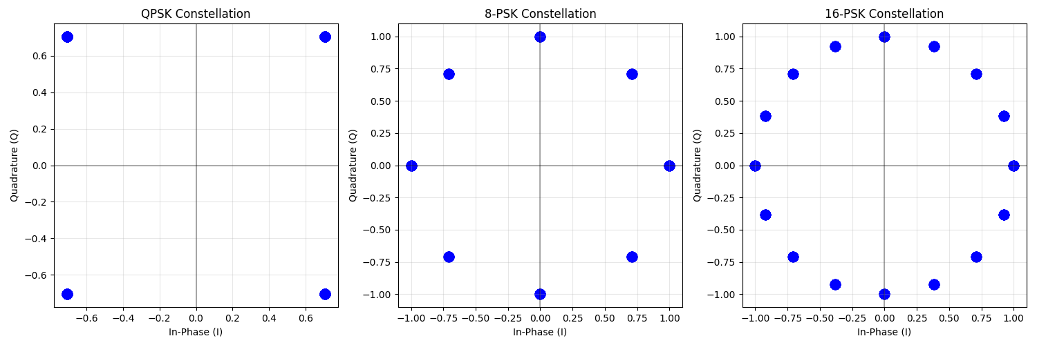
Visualize Constellation Diagrams

fig, axs = plt.subplots(1, 3, figsize=(15, 5))

# QPSK constellation
plot_constellation(qpsk_symbols.flatten(), title="QPSK Constellation", marker="o", ax=axs[0])
axs[0].grid(True)

# 8-PSK constellation
plot_constellation(psk8_symbols.flatten(), title="8-PSK Constellation", marker="o", ax=axs[1])
axs[1].grid(True)

# 16-PSK constellation
plot_constellation(psk16_symbols.flatten(), title="16-PSK Constellation", marker="o", ax=axs[2])
axs[2].grid(True)

plt.tight_layout()
plt.show()

Compare Symbol Distance

Higher-order PSK constellations have reduced distance between adjacent symbols

fig = plt.figure(figsize=(15, 5))

# Calculate min distances between adjacent symbols
# QPSK: symbols at 0, 90, 180, 270 degrees -> min dist = sqrt(2)
# 8-PSK: symbols at 0, 45, 90... degrees -> min dist = 2*sin(pi/8)
# 16-PSK: symbols at 0, 22.5, 45... degrees -> min dist = 2*sin(pi/16)

qpsk_min_dist = 2 * np.sin(np.pi / 4)
psk8_min_dist = 2 * np.sin(np.pi / 8)
psk16_min_dist = 2 * np.sin(np.pi / 16)

# Plot with normalized radius showing minimum distances
ax1 = fig.add_subplot(131)
circle = plt.Circle((0, 0), 1, fill=False, linestyle="--", color="gray")
ax1.add_patch(circle)
ax1.scatter([1, 0, -1, 0], [0, 1, 0, -1], color="blue")
ax1.plot([0, 1], [0, 0], color="red", linewidth=2)
ax1.set_xlim(-1.2, 1.2)
ax1.set_ylim(-1.2, 1.2)
ax1.grid(True)
ax1.set_title(f"QPSK\nMin Distance = {qpsk_min_dist:.3f}")
ax1.set_aspect("equal")

ax2 = fig.add_subplot(132)
circle = plt.Circle((0, 0), 1, fill=False, linestyle="--", color="gray")
ax2.add_patch(circle)
theta = np.linspace(0, 2 * np.pi, 8, endpoint=False)
ax2.scatter(np.cos(theta), np.sin(theta), color="blue")
ax2.plot([0, np.cos(0)], [0, np.sin(0)], color="red", linewidth=2)
ax2.plot([0, np.cos(np.pi / 4)], [0, np.sin(np.pi / 4)], color="red", linewidth=2)
ax2.set_xlim(-1.2, 1.2)
ax2.set_ylim(-1.2, 1.2)
ax2.grid(True)
ax2.set_title(f"8-PSK\nMin Distance = {psk8_min_dist:.3f}")
ax2.set_aspect("equal")

ax3 = fig.add_subplot(133)
circle = plt.Circle((0, 0), 1, fill=False, linestyle="--", color="gray")
ax3.add_patch(circle)
theta = np.linspace(0, 2 * np.pi, 16, endpoint=False)
ax3.scatter(np.cos(theta), np.sin(theta), color="blue")
ax3.plot([0, np.cos(0)], [0, np.sin(0)], color="red", linewidth=2)
ax3.plot([0, np.cos(np.pi / 8)], [0, np.sin(np.pi / 8)], color="red", linewidth=2)
ax3.set_xlim(-1.2, 1.2)
ax3.set_ylim(-1.2, 1.2)
ax3.grid(True)
ax3.set_title(f"16-PSK\nMin Distance = {psk16_min_dist:.3f}")
ax3.set_aspect("equal")

plt.tight_layout()
plt.show()

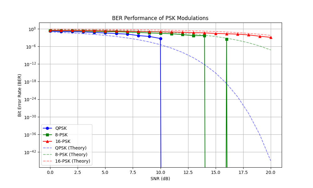
Performance in AWGN Channel

Compare BER for different PSK orders in AWGN

snr_db_range = np.arange(0, 21, 1)
ber_qpsk = []
ber_psk8 = []
ber_psk16 = []

# Initialize BER metric
ber_metric = BER()

for snr_db in snr_db_range:
    # Calculate noise power and create AWGN channel
    noise_power = snr_to_noise_power(1.0, snr_db)
    channel = AWGNChannel(avg_noise_power=noise_power)

    # QPSK transmission
    received_qpsk = channel(qpsk_symbols)
    demod_bits_qpsk = qpsk_demod(received_qpsk)
    ber_qpsk.append(ber_metric(demod_bits_qpsk, qpsk_bits).item())

    # 8-PSK transmission
    received_psk8 = channel(psk8_symbols)
    demod_bits_psk8 = psk8_demod(received_psk8)
    ber_psk8.append(ber_metric(demod_bits_psk8, psk8_bits).item())

    # 16-PSK transmission
    received_psk16 = channel(psk16_symbols)
    demod_bits_psk16 = psk16_demod(received_psk16)
    ber_psk16.append(ber_metric(demod_bits_psk16, psk16_bits).item())

# Plot BER vs SNR
plt.figure(figsize=(10, 6))
plt.semilogy(snr_db_range, ber_qpsk, "b-", marker="o", label="QPSK")
plt.semilogy(snr_db_range, ber_psk8, "g-", marker="s", label="8-PSK")
plt.semilogy(snr_db_range, ber_psk16, "r-", marker="^", label="16-PSK")

# Approximate theoretical bounds
snr_lin = 10 ** (snr_db_range / 10)
theoretical_ber_qpsk = torch.erfc(torch.sqrt(torch.tensor(snr_lin))) / 2
theoretical_ber_8psk = torch.erfc(torch.sqrt(torch.tensor(snr_lin) * np.sin(np.pi / 8) ** 2))
theoretical_ber_16psk = torch.erfc(torch.sqrt(torch.tensor(snr_lin) * np.sin(np.pi / 16) ** 2))

plt.semilogy(snr_db_range, theoretical_ber_qpsk, "b--", alpha=0.5, label="QPSK (Theory)")
plt.semilogy(snr_db_range, theoretical_ber_8psk, "g--", alpha=0.5, label="8-PSK (Theory)")
plt.semilogy(snr_db_range, theoretical_ber_16psk, "r--", alpha=0.5, label="16-PSK (Theory)")

plt.grid(True)
plt.xlabel("SNR (dB)")
plt.ylabel("Bit Error Rate (BER)")
plt.title("BER Performance of PSK Modulations")
plt.legend()
plt.show()

Effect of Noise on Constellations

Let’s visualize how noise affects the constellation diagrams at a fixed SNR

test_snr_db = 15  # 15 dB SNR
noise_power = snr_to_noise_power(1.0, test_snr_db)
channel = AWGNChannel(avg_noise_power=noise_power)

# Generate new test data
test_n_symbols = 500
test_qpsk_bits = torch.randint(0, 2, (1, 2 * test_n_symbols))
test_psk8_bits = torch.randint(0, 2, (1, 3 * test_n_symbols))
test_psk16_bits = torch.randint(0, 2, (1, 4 * test_n_symbols))

test_qpsk = qpsk_mod(test_qpsk_bits)
test_psk8 = psk8_mod(test_psk8_bits)
test_psk16 = psk16_mod(test_psk16_bits)

received_qpsk = channel(test_qpsk)
received_psk8 = channel(test_psk8)
received_psk16 = channel(test_psk16)

# Plot noisy constellations
fig, axs = plt.subplots(1, 3, figsize=(15, 5))

plot_constellation(received_qpsk.flatten(), title=f"QPSK at {test_snr_db} dB SNR", marker=".", ax=axs[0])
axs[0].grid(True)

plot_constellation(received_psk8.flatten(), title=f"8-PSK at {test_snr_db} dB SNR", marker=".", ax=axs[1])
axs[1].grid(True)

plot_constellation(received_psk16.flatten(), title=f"16-PSK at {test_snr_db} dB SNR", marker=".", ax=axs[2])
axs[2].grid(True)

plt.tight_layout()
plt.show()

Soft Demodulation

Demonstrate soft decision demodulation (LLR output)

test_snr_db = 10  # 10 dB SNR
noise_power = snr_to_noise_power(1.0, test_snr_db)

# Generate simple test sequence
test_qpsk_bits = torch.tensor([[0, 0, 1, 1, 0, 1, 1, 0, 0, 1]])
test_qpsk = qpsk_mod(test_qpsk_bits)

# Add noise
channel = AWGNChannel(avg_noise_power=noise_power)
received_qpsk = channel(test_qpsk)

# Demodulate with hard and soft decision
hard_bits = qpsk_demod(received_qpsk)
soft_llrs = qpsk_demod(received_qpsk, noise_var=noise_power)

# Print results for comparison
print("\nDemodulation Results:")
print("Original bits:", test_qpsk_bits.numpy().flatten())
print("Hard decisions:", hard_bits.numpy().flatten().astype(int))
print("Soft LLRs:", soft_llrs.numpy().flatten())

# Create figure with two subplots
plt.figure(figsize=(15, 6))

# Plot received symbols and constellation
plt.subplot(1, 2, 1)
# Plot the received symbols
plt.scatter(received_qpsk.real.numpy(), received_qpsk.imag.numpy(), c="blue", marker="o", label="Received", alpha=0.6)

# Add original constellation points for reference
qpsk_const = qpsk_mod.constellation
plt.scatter(qpsk_const.real.numpy(), qpsk_const.imag.numpy(), c="red", marker="x", s=100, label="Constellation Points")

# Add bit labels to constellation points
for i, point in enumerate(qpsk_const):
    bits = "".join(str(int(b)) for b in qpsk_mod.bit_patterns[i])
    plt.annotate(bits, (point.real + 0.1, point.imag + 0.1))

plt.grid(True)
plt.xlabel("In-Phase")
plt.ylabel("Quadrature")
plt.title(f"QPSK Received Symbols at {test_snr_db} dB SNR")
plt.legend()
plt.axis("equal")

# Plot LLR values
plt.subplot(1, 2, 2)
x = np.arange(len(soft_llrs.numpy().flatten()))
llr_values = soft_llrs.numpy().flatten()
plt.stem(x, llr_values)  # Removed deprecated parameter
plt.axhline(y=0, color="r", linestyle="--", alpha=0.3)
plt.grid(True)
plt.xlabel("LLR Index")
plt.ylabel("LLR Value")
plt.title("Soft Decision Log-Likelihood Ratios (LLRs)")

# Add decision threshold reference
plt.axhline(y=0, color="r", linestyle="--", label="Decision Threshold")
plt.legend()

plt.tight_layout()
plt.show()

Demodulation Results:
Original bits: [0 0 1 1 0 1 1 0 0 1]
Hard decisions: [0 0 1 1 0 1 1 0 0 1]
Soft LLRs: [-16.662338 -12.416273  17.974085  22.315212 -34.97273   28.40015
  31.671106 -30.650873 -25.182978  27.120493]

Efficiency vs. Performance Trade-off

Calculate minimum required SNR to achieve target BER for each modulation

target_ber = 1e-5
required_snr_qpsk = np.interp(target_ber, theoretical_ber_qpsk.numpy()[::-1], snr_db_range[::-1])
required_snr_8psk = np.interp(target_ber, theoretical_ber_8psk.numpy()[::-1], snr_db_range[::-1])
required_snr_16psk = np.interp(target_ber, theoretical_ber_16psk.numpy()[::-1], snr_db_range[::-1])

# Create a bar chart of spectral efficiency vs required SNR
plt.figure(figsize=(10, 6))
modulations = ["QPSK", "8-PSK", "16-PSK"]
spectral_efficiencies = [2, 3, 4]  # bits/s/Hz
required_snrs = [required_snr_qpsk, required_snr_8psk, required_snr_16psk]

bars = plt.bar(modulations, spectral_efficiencies, width=0.5)
plt.ylabel("Spectral Efficiency (bits/s/Hz)")
plt.title(f"Spectral Efficiency vs Required SNR for BER = {target_ber}")

# Add required SNR as text on each bar
for i, (bar, snr) in enumerate(zip(bars, required_snrs)):
    plt.text(i, bar.get_height() + 0.1, f"Required SNR: {snr:.1f} dB", ha="center", va="bottom", fontweight="bold")

plt.tight_layout()
plt.show()

Conclusion

This example demonstrated:

1. Implementation of higher-order PSK modulation (8-PSK, 16-PSK) using Kaira

2. Visualization of constellation diagrams for different PSK orders

3. Analysis of minimum symbol distances and their impact on performance

4. BER performance comparison in AWGN channels

5. Efficiency vs. performance trade-offs

Key observations:

• Higher-order PSK schemes increase spectral efficiency (bits/s/Hz)

• The increased efficiency comes at the cost of reduced noise immunity

• Minimum distance between symbols decreases as modulation order increases

• Higher-order PSK requires higher SNR to achieve the same BER

• This illustrates the fundamental trade-off between efficiency and robustness