Modulation Schemes for Digital Communication Systems

This example demonstrates various digital modulation schemes available in Kaira. Modulation is the process of encoding information onto carrier signals, which is a fundamental component of any communication system.

We’ll explore different modulation techniques and visualize their constellation diagrams, bit error rates, and spectral properties.

import matplotlib.pyplot as plt
import numpy as np
import seaborn as sns
import torch
from matplotlib.gridspec import GridSpec

from kaira.channels import AWGNChannel
from kaira.modulations import (  # Modulators; Demodulators
    BPSKDemodulator,
    BPSKModulator,
    PAMDemodulator,
    PAMModulator,
    PSKDemodulator,
    PSKModulator,
    QAMDemodulator,
    QAMModulator,
    QPSKDemodulator,
    QPSKModulator,
)

# Set visual style for better presentation
plt.style.use("seaborn-v0_8-whitegrid")
sns.set_context("notebook", font_scale=1.2)
colors = sns.color_palette("viridis", 6)
accent_colors = sns.color_palette("Set2", 8)

# Set random seed for reproducibility
torch.manual_seed(42)
np.random.seed(42)


# Helper function to convert integers to binary arrays (replacement for torch.unpackbits)
def int_to_bits(n, num_bits):
    """Convert integer to binary representation as tensor.

    Args:
        n: Integer or tensor of integers
        num_bits: Number of bits to use for representation

    Returns:
        Tensor with binary representation (each bit as a separate value)
    """
    if isinstance(n, torch.Tensor):
        result = torch.zeros((n.shape[0], num_bits), dtype=torch.float32)
        for i in range(n.shape[0]):
            val = n[i].item()
            for j in range(num_bits):
                result[i, num_bits - j - 1] = (val >> j) & 1
        return result
    else:
        result = torch.zeros(num_bits, dtype=torch.float32)
        for j in range(num_bits):
            result[num_bits - j - 1] = (n >> j) & 1
        return result


# Add a utility function to safely convert potentially complex values to real for plotting
def safe_to_real(value):
    """Convert potentially complex values to real for plotting."""
    if isinstance(value, torch.Tensor):
        if torch.is_complex(value):
            return value.real
    elif isinstance(value, np.ndarray):
        if np.iscomplexobj(value):
            return value.real
    return value


# Add a utility function to safely compute absolute values of potentially complex numbers
def safe_abs(value):
    """Safely compute absolute value, handling complex numbers appropriately."""
    if isinstance(value, torch.Tensor):
        if torch.is_complex(value):
            return torch.abs(value)
    elif isinstance(value, np.ndarray):
        if np.iscomplexobj(value):
            return np.abs(value)
    return np.abs(value)  # Default to numpy abs for real values


# Modem class to simplify working with modulator and demodulator pairs
class Modem:
    """A class that combines a modulator and demodulator.

    This provides a simple interface for working with modulation schemes.
    """

    def __init__(self, modulator, demodulator, soft_output=False):
        """Initialize the modem.

        Args:
            modulator: A modulator instance
            demodulator: A demodulator instance
            soft_output: Whether to produce soft decisions (LLRs) when demodulating
        """
        self.modulator = modulator
        self.demodulator = demodulator
        self.soft_output = soft_output

    def modulate(self, bits):
        """Modulate bits to symbols.

        Args:
            bits: Input tensor of bits

        Returns:
            Tensor of modulated symbols
        """
        return self.modulator(bits)

    def demodulate(self, symbols, noise_var=None):
        """Demodulate symbols to bits.

        Args:
            symbols: Input tensor of symbols
            noise_var: Noise variance for soft demodulation

        Returns:
            Tensor of demodulated bits
        """
        if self.soft_output:
            if noise_var is None:
                noise_var = 1.0  # Default noise variance
            return self.demodulator(symbols, noise_var)
        else:
            return self.demodulator(symbols)


# Add a utility function to safely create scatter plots with potentially complex values
def safe_scatter(ax, x, y, *args, **kwargs):
    """Create a scatter plot ensuring x and y values are real.

    Args:
        ax: Matplotlib axis
        x: x-coordinates (potentially complex)
        y: y-coordinates (potentially complex)
        *args, **kwargs: Additional arguments passed to scatter

    Returns:
        The scatter plot instance
    """
    x_real = safe_to_real(x)
    y_real = safe_to_real(y)
    return ax.scatter(x_real, y_real, *args, **kwargs)


# Add a utility function to safely plot lines with potentially complex values
def safe_plot(ax, x, y, *args, **kwargs):
    """Create a line plot ensuring x and y values are real.

    Args:
        ax: Matplotlib axis
        x: x-coordinates (potentially complex)
        y: y-coordinates (potentially complex)
        *args, **kwargs: Additional arguments passed to plot

    Returns:
        The line plot instance
    """
    x_real = safe_to_real(x)
    y_real = safe_to_real(y)
    return ax.plot(x_real, y_real, *args, **kwargs)

Introduction to Digital Modulation

Digital modulation maps discrete information (bits) to analog signals for transmission. Different modulation schemes offer different trade-offs between:

• Spectral efficiency (bits per Hz)

• Power efficiency (energy per bit)

• Robustness to noise and interference

• Implementation complexity

Below, we’ll visualize and compare key modulation schemes supported by Kaira.

# Create a list of modulation schemes to compare
modulation_schemes: list[tuple[str, Modem, int]] = [
    ("BPSK", Modem(BPSKModulator(), BPSKDemodulator(), soft_output=False), 1),
    ("QPSK", Modem(QPSKModulator(), QPSKDemodulator(), soft_output=False), 2),
    ("8-PSK", Modem(PSKModulator(order=8), PSKDemodulator(order=8), soft_output=False), 3),
    ("16-QAM", Modem(QAMModulator(order=16), QAMDemodulator(order=16), soft_output=False), 4),
    ("64-QAM", Modem(QAMModulator(order=64), QAMDemodulator(order=64), soft_output=False), 6),
    ("8-PAM", Modem(PAMModulator(order=8), PAMDemodulator(order=8), soft_output=False), 3),
]

# Create a figure to display constellation diagrams
fig = plt.figure(figsize=(18, 12))
gs = GridSpec(2, 3, figure=fig)

# Generate constellation diagrams for each modulation scheme
for i, (name, modulation, bits_per_symbol) in enumerate(modulation_schemes):
    # Create subplot
    ax = fig.add_subplot(gs[i // 3, i % 3])

    # Generate all possible symbols
    num_symbols = 2**bits_per_symbol
    indices = torch.arange(num_symbols)
    bits = int_to_bits(indices, bits_per_symbol)

    # Modulate the bits
    symbols = modulation.modulate(bits)

    # For plotting, ensure we properly handle complex symbols
    # For 1D modulations, set the imaginary part to zero
    if symbols.shape[1] == 1:
        symbol_real = safe_to_real(symbols[:, 0]).numpy()
        symbol_imag = np.zeros_like(symbol_real)
    else:
        symbol_real = safe_to_real(symbols[:, 0]).numpy()
        symbol_imag = safe_to_real(symbols[:, 1]).numpy() if symbols.shape[1] > 1 else symbols[:, 0].imag.numpy()

    # Plot the constellation
    scatter = safe_scatter(ax, symbol_real, symbol_imag, s=100, alpha=0.7, c=np.arange(len(symbols)), cmap="viridis")

    # Add bit labels to points
    for j in range(len(bits)):
        bit_str = "".join(bits[j].numpy().astype(int).astype(str))
        ax.annotate(bit_str, (symbol_real[j], symbol_imag[j]), fontsize=8, ha="right", va="bottom")

    # Draw connecting lines to origin for PSK modulations
    if "PSK" in name:
        for j in range(len(symbols)):
            safe_plot(ax, [0, safe_to_real(symbols[j, 0]).numpy()], [0, safe_to_real(symbols[j, 1]).numpy() if symbols.shape[1] > 1 else 0], "gray", alpha=0.3, linestyle="--")

    # Draw grid lines for QAM modulations
    if "QAM" in name:
        unique_x = np.sort(np.unique(safe_to_real(symbols[:, 0]).numpy()))
        if symbols.shape[1] > 1:  # Check if symbols have a second dimension
            unique_y = np.sort(np.unique(safe_to_real(symbols[:, 1]).numpy()))
            for y in unique_y:
                ax.axhline(y, color="gray", alpha=0.2, linestyle="-")
        for x in unique_x:
            ax.axvline(x, color="gray", alpha=0.2, linestyle="-")

    # Add reference circle for PSK modulations
    if "PSK" in name:
        radius = np.abs(safe_to_real(symbols[0, 0]).numpy())  # All PSK symbols have same radius
        circle = plt.Circle((0, 0), radius, fill=False, color="gray", linestyle="--", alpha=0.5)
        ax.add_patch(circle)

    # Add title and grid
    ax.set_title(f"{name} ({bits_per_symbol} bits/symbol)", fontsize=14, fontweight="bold")
    ax.grid(True, alpha=0.3)
    ax.set_xlabel("In-phase (I)", fontsize=12)
    ax.set_ylabel("Quadrature (Q)", fontsize=12)

    # Ensure equal aspect ratio
    ax.set_aspect("equal")

    # Set axis limits to make visualization consistent
    max_val = max(np.abs(symbols.numpy()).max() * 1.2, 1.5)
    ax.set_xlim(-max_val, max_val)
    ax.set_ylim(-max_val, max_val)

    # Add origin lines
    ax.axhline(y=0, color="black", alpha=0.5, linestyle="-")
    ax.axvline(x=0, color="black", alpha=0.5, linestyle="-")

plt.suptitle("Constellation Diagrams for Different Modulation Schemes", fontsize=16, fontweight="bold")
plt.tight_layout(rect=(0, 0.03, 1, 0.97))

Calculating Bit Error Rate (BER) for Different Schemes

The Bit Error Rate (BER) is a key performance metric for digital communication systems. It measures the number of bit errors divided by the total number of transmitted bits. Let’s compare the BER performance of different modulation schemes over varying SNR.

# Setup simulation parameters
snr_db_range = np.arange(0, 21, 2)  # SNR range from 0 to 20 dB
num_bits = 100000  # Number of bits to simulate for each scheme and SNR
ber_results: dict[str, list[float]] = {name: [] for name, _, _ in modulation_schemes}

# Create AWGN channel for simulation
channel = AWGNChannel(snr_db=10.0)  # Initial SNR will be updated in the loop

# Generate random bits for transmission
for name, modulation, bits_per_symbol in modulation_schemes:
    print(f"Simulating BER for {name}...")

    # Calculate required number of symbols
    num_symbols = num_bits // bits_per_symbol

    # Generate random bits
    input_bits = torch.randint(0, 2, (num_symbols, bits_per_symbol), dtype=torch.float32)

    for snr_db in snr_db_range:
        # Update channel SNR
        channel.snr_db = float(snr_db)

        # Modulate bits to symbols
        tx_symbols = modulation.modulate(input_bits)

        # Pass through the noisy channel
        rx_symbols = channel(tx_symbols)

        # Demodulate the received symbols
        rx_bits = modulation.demodulate(rx_symbols)

        # Calculate bit error rate
        bit_errors = (rx_bits != input_bits).sum().item()
        ber = bit_errors / (num_symbols * bits_per_symbol)

        # Store result (use a small minimum value for log plotting)
        ber_results[name].append(max(ber, 1e-7))

Simulating BER for BPSK...
Simulating BER for QPSK...
Simulating BER for 8-PSK...
Simulating BER for 16-QAM...
Simulating BER for 64-QAM...
Simulating BER for 8-PAM...

BER Performance Visualization

Now let’s create an informative plot showing the BER vs SNR performance.

plt.figure(figsize=(12, 8))

# Plot BER curves
for i, (name, _, bits_per_symbol) in enumerate(modulation_schemes):
    plt.semilogy(snr_db_range, ber_results[name], "o-", linewidth=2.5, markersize=8, label=f"{name} ({bits_per_symbol} bits/symbol)", color=accent_colors[i])


# Add theoretical BER curves for common modulations
def q_function(x):
    """Q-function approximation."""
    return 0.5 * np.exp(-0.5 * x**2)


# Add theoretical BPSK BER curve
snr_lin = 10 ** (snr_db_range / 10)
theo_bpsk_ber = q_function(np.sqrt(2 * snr_lin))
plt.semilogy(snr_db_range, theo_bpsk_ber, "k--", alpha=0.7, linewidth=1.5, label="BPSK (Theoretical)")

# Add theoretical QPSK BER curve (same as BPSK in AWGN)
plt.semilogy(snr_db_range, theo_bpsk_ber, "k:", alpha=0.7, linewidth=1.5, label="QPSK (Theoretical)")

# Format the plot
plt.grid(True, which="both", linestyle="--", alpha=0.7)
plt.xlabel("Signal-to-Noise Ratio (SNR) [dB]", fontsize=14)
plt.ylabel("Bit Error Rate (BER)", fontsize=14)
plt.title("BER Performance Comparison of Modulation Schemes", fontsize=16, fontweight="bold")
plt.legend(loc="best", fontsize=12)
plt.tight_layout()

# Add annotations to highlight important aspects
plt.annotate("Higher spectral efficiency\noften means worse BER performance", xy=(14, 1e-2), xytext=(14, 1e-1), arrowprops=dict(arrowstyle="->", connectionstyle="arc3,rad=0.3", color="red"), bbox=dict(boxstyle="round,pad=0.3", fc="white", ec="red", alpha=0.8), fontsize=12, ha="center")

plt.annotate("Most robust\nscheme", xy=(14, theo_bpsk_ber[7]), xytext=(6, 1e-6), arrowprops=dict(arrowstyle="->", connectionstyle="arc3,rad=-0.3", color="green"), bbox=dict(boxstyle="round,pad=0.3", fc="white", ec="green", alpha=0.8), fontsize=12)

Text(6, 1e-06, 'Most robust\nscheme')

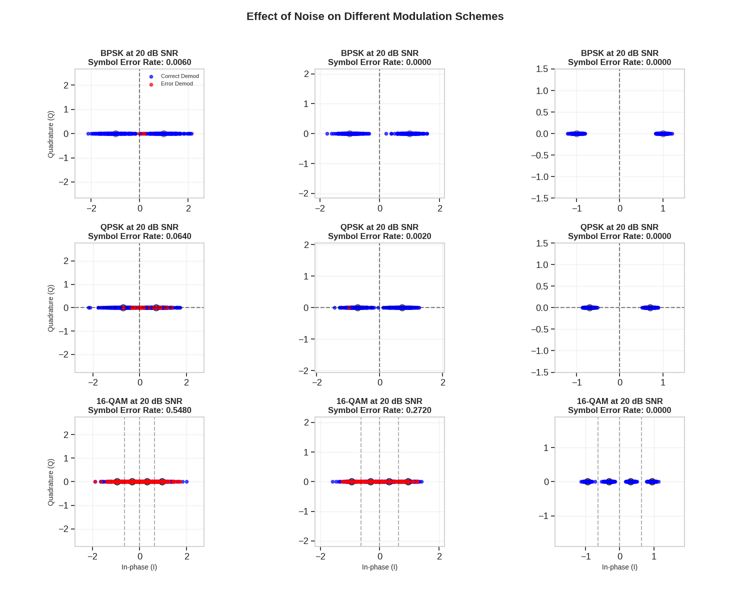
Visualizing the Effects of Noise on Modulation Schemes

Let’s examine how noise affects different modulation schemes visually.

# Select modulation schemes for this visualization
vis_schemes = [("BPSK", Modem(BPSKModulator(), BPSKDemodulator(), soft_output=False), 1), ("QPSK", Modem(QPSKModulator(), QPSKDemodulator(), soft_output=False), 2), ("16-QAM", Modem(QAMModulator(order=16), QAMDemodulator(order=16), soft_output=False), 4)]

# Define SNR values to visualize
snr_values = [5, 10, 20]  # Low, medium, high SNR in dB

# Create figure with subplots
fig = plt.figure(figsize=(15, 12))
gs = GridSpec(len(vis_schemes), len(snr_values), figure=fig)

# Generate the test data - same symbols for all tests
num_test_symbols = 500
np.random.seed(42)  # Ensure reproducibility

for i, (name, modulation, bits_per_symbol) in enumerate(vis_schemes):
    # Generate random bits (same for all SNRs)
    input_bits = torch.randint(0, 2, (num_test_symbols, bits_per_symbol), dtype=torch.float32)

    # Modulate bits to symbols
    tx_symbols = modulation.modulate(input_bits)

    for j, snr_db_value in enumerate(snr_values):
        # Create subplot
        ax = fig.add_subplot(gs[i, j])

        # Update channel SNR
        channel = AWGNChannel(snr_db=float(snr_db_value))

        # Pass through noisy channel
        rx_symbols = channel(tx_symbols)

        # Demodulate received symbols
        rx_bits = modulation.demodulate(rx_symbols)

        # Calculate symbol errors
        if bits_per_symbol == 1:  # Handle BPSK separately since it's 1D
            sym_errors = (rx_bits != input_bits).any(dim=1)
        else:
            sym_errors = (rx_bits != input_bits).any(dim=1)

        # Plot the original constellation points as reference
        # Use smaller markers for the reference constellation
        if bits_per_symbol == 1:  # BPSK case (1D)
            unique_symbols = modulation.modulate(torch.tensor([[0.0], [1.0]]))
            safe_scatter(ax, safe_to_real(unique_symbols[:, 0]).numpy(), np.zeros_like(unique_symbols[:, 0].numpy()), s=80, color="gray", alpha=0.5, marker="o", edgecolor="black")
        else:
            unique_bits = torch.zeros((2**bits_per_symbol, bits_per_symbol))
            for k in range(2**bits_per_symbol):
                unique_bits[k] = torch.tensor([(k >> bit_position) & 1 for bit_position in range(bits_per_symbol - 1, -1, -1)])
            unique_symbols = modulation.modulate(unique_bits)

            # For 1D modulations, handle differently
            if unique_symbols.shape[1] == 1:
                safe_scatter(ax, safe_to_real(unique_symbols[:, 0]).numpy(), np.zeros_like(unique_symbols[:, 0].numpy()), s=80, color="gray", alpha=0.5, marker="o", edgecolor="black")
            else:
                safe_scatter(ax, safe_to_real(unique_symbols[:, 0]).numpy(), safe_to_real(unique_symbols[:, 1]).numpy(), s=80, color="gray", alpha=0.5, marker="o", edgecolor="black")

        # Plot the received symbols
        if bits_per_symbol == 1 or rx_symbols.shape[1] == 1:  # Handle any 1D modulation
            correct = safe_scatter(ax, safe_to_real(rx_symbols[~sym_errors, 0]).numpy(), np.zeros_like(rx_symbols[~sym_errors, 0].numpy()), s=20, alpha=0.7, c="blue", label="Correct Demod")
            errors = safe_scatter(ax, safe_to_real(rx_symbols[sym_errors, 0]).numpy(), np.zeros_like(rx_symbols[sym_errors, 0].numpy()), s=20, alpha=0.7, c="red", label="Error Demod")
        else:
            correct = safe_scatter(ax, safe_to_real(rx_symbols[~sym_errors, 0]).numpy(), safe_to_real(rx_symbols[~sym_errors, 1]).numpy(), s=20, alpha=0.7, c="blue", label="Correct Demod")
            errors = safe_scatter(ax, safe_to_real(rx_symbols[sym_errors, 0]).numpy(), safe_to_real(rx_symbols[sym_errors, 1]).numpy(), s=20, alpha=0.7, c="red", label="Error Demod")

        # Add decision boundaries
        if name == "BPSK":
            ax.axvline(x=0, color="black", linestyle="--", alpha=0.5)
        elif name == "QPSK":
            ax.axhline(y=0, color="black", linestyle="--", alpha=0.5)
            ax.axvline(x=0, color="black", linestyle="--", alpha=0.5)
        elif name == "16-QAM":
            # QAM decision boundaries are equally spaced between constellation points
            symbs = unique_symbols.numpy()
            unique_x = np.sort(np.unique(safe_to_real(symbs[:, 0])))

            # Check if the modulation is 1D or 2D before accessing second dimension
            if symbs.shape[1] > 1:  # 2D modulation
                unique_y = np.sort(np.unique(safe_to_real(symbs[:, 1])))

                # Compute decision boundaries between symbol points
                x_boundaries = (unique_x[:-1] + unique_x[1:]) / 2
                y_boundaries = (unique_y[:-1] + unique_y[1:]) / 2

                for x in x_boundaries:
                    ax.axvline(x=x, color="black", linestyle="--", alpha=0.3)
                for y in y_boundaries:
                    ax.axhline(y=y, color="black", linestyle="--", alpha=0.3)
            else:  # 1D modulation
                # Compute decision boundaries between symbol points only for x-axis
                x_boundaries = (unique_x[:-1] + unique_x[1:]) / 2

                for x in x_boundaries:
                    ax.axvline(x=x, color="black", linestyle="--", alpha=0.3)

        # Calculate and display error rate
        error_rate = sym_errors.sum().item() / num_test_symbols

        # Add title and grid
        ax.set_title(f"{name} at {snr_db} dB SNR\nSymbol Error Rate: {error_rate:.4f}", fontsize=12, fontweight="bold")
        ax.grid(True, alpha=0.3)

        # Set axis labels only for the bottom row and leftmost column
        if i == len(vis_schemes) - 1:
            ax.set_xlabel("In-phase (I)", fontsize=10)
        if j == 0:
            ax.set_ylabel("Quadrature (Q)", fontsize=10)

        # Ensure equal aspect ratio
        ax.set_aspect("equal")

        # Set reasonable axis limits
        max_val = max(np.abs(rx_symbols.numpy()).max() * 1.2, 1.5)
        ax.set_xlim(-max_val, max_val)
        ax.set_ylim(-max_val, max_val)

        # Add legend only for the first plot
        if i == 0 and j == 0:
            ax.legend(fontsize=8, loc="upper right")

plt.suptitle("Effect of Noise on Different Modulation Schemes", fontsize=16, fontweight="bold")
plt.tight_layout(rect=(0, 0.03, 1, 0.97))

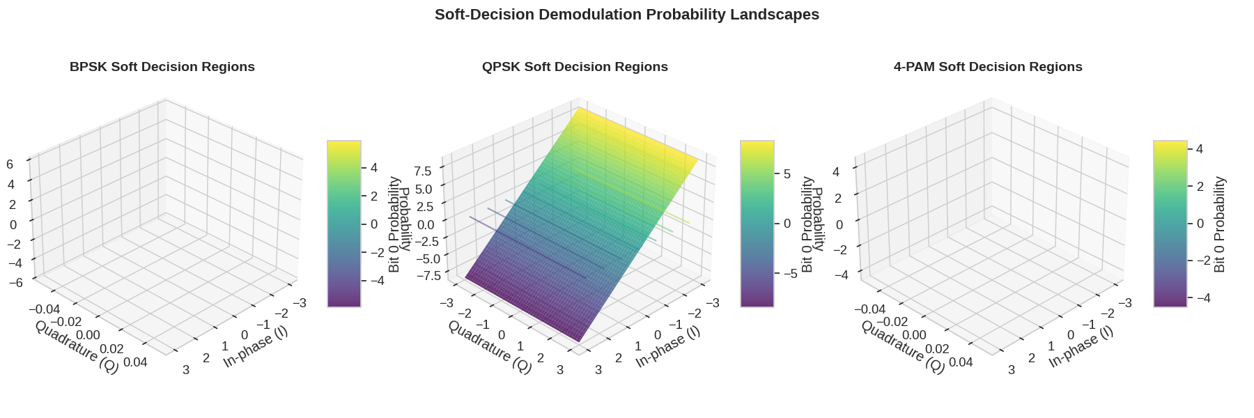
3D Visualization of Soft Decision Boundaries

For soft-decision demodulation, the output isn’t just bits, but probabilities. Let’s visualize this with a 3D plot showing the decision regions.

# Setup for 3D visualization
plt.figure(figsize=(18, 6))

# Choose modulation schemes for soft-decision visualization
soft_modulations = [("BPSK", Modem(BPSKModulator(), BPSKDemodulator(), soft_output=True)), ("QPSK", Modem(QPSKModulator(), QPSKDemodulator(), soft_output=True)), ("4-PAM", Modem(PAMModulator(order=4), PAMDemodulator(order=4), soft_output=True))]

# Create a grid of points to evaluate the soft decision functions
x = np.linspace(-3, 3, 100)
y = np.linspace(-3, 3, 100)
X, Y = np.meshgrid(x, y)
points = np.column_stack((X.flatten(), Y.flatten()))

for i, (name, modulation) in enumerate(soft_modulations):
    ax = plt.subplot(1, 3, i + 1, projection="3d")

    # Create input tensor
    input_tensor = torch.tensor(points, dtype=torch.float32)

    # For 1D modulations, we only use the first dimension
    if name in ["BPSK", "4-PAM"]:
        input_tensor = input_tensor[:, 0:1]

    # Get soft bit probabilities
    with torch.no_grad():
        soft_bits = modulation.demodulate(input_tensor)

    # Plot the first bit probability as a 3D surface
    if name in ["BPSK", "4-PAM"]:
        # For 1D modulations, plot along the x-axis only
        Z = np.zeros_like(X)
        Z[:, :] = safe_to_real(soft_bits[:, 0]).numpy().reshape(X.shape)
        surf = ax.plot_surface(X, np.zeros_like(Y), Z, cmap="viridis", alpha=0.8, linewidth=0, antialiased=True)  # type: ignore[attr-defined]
        ax.contour(X, np.zeros_like(Y), Z, zdir="z", offset=0, cmap="viridis", alpha=0.5)
    else:
        # For 2D modulations, use the full grid
        Z = safe_to_real(soft_bits[:, 0]).numpy().reshape(X.shape)
        surf = ax.plot_surface(X, Y, Z, cmap="viridis", alpha=0.8, linewidth=0, antialiased=True)  # type: ignore[attr-defined]
        ax.contour(X, Y, Z, zdir="z", offset=0, cmap="viridis", alpha=0.5)

    # Add a colorbar
    plt.colorbar(surf, ax=ax, shrink=0.5, aspect=5, label="Bit 0 Probability")

    # Set labels and title
    ax.set_xlabel("In-phase (I)")
    ax.set_ylabel("Quadrature (Q)")
    ax.set_zlabel("Probability")  # type: ignore[attr-defined]
    ax.set_title(f"{name} Soft Decision Regions", fontsize=14, fontweight="bold")

    # Set reasonable view angle
    ax.view_init(elev=30, azim=45)  # type: ignore[attr-defined]

plt.suptitle("Soft-Decision Demodulation Probability Landscapes", fontsize=16, fontweight="bold")
plt.tight_layout(rect=(0, 0.03, 1, 0.97))

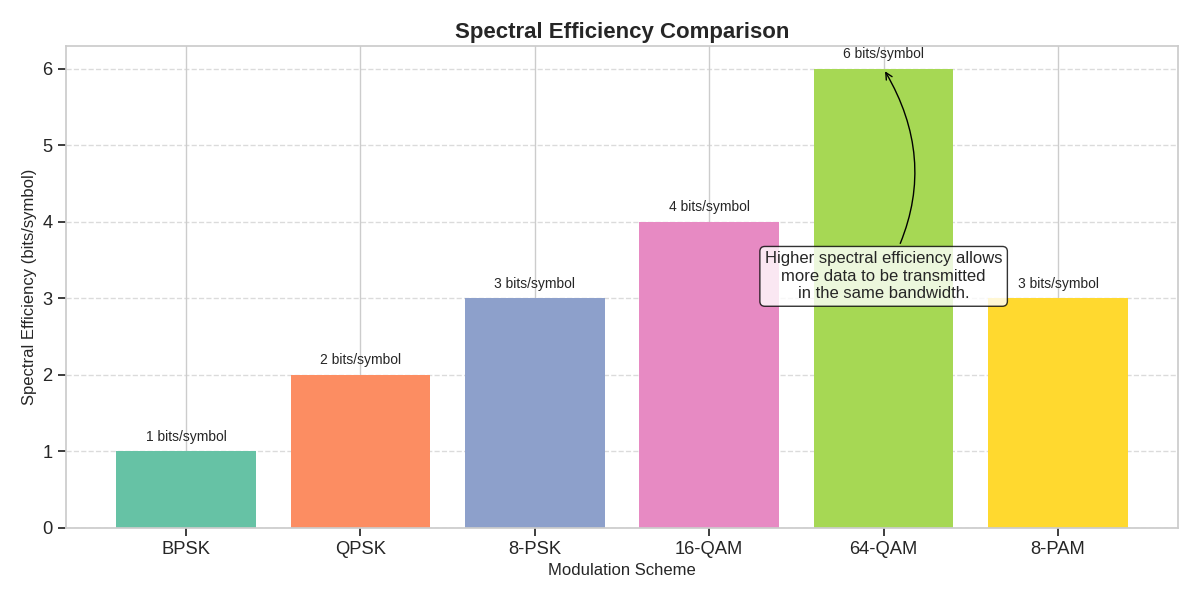
Spectral Efficiency Comparison

Let’s visualize the spectral efficiency (bits/s/Hz) of different modulation schemes.

# Calculate spectral efficiency (bits per symbol) for each scheme
spectral_efficiency = [bits for _, _, bits in modulation_schemes]
scheme_names = [name for name, _, _ in modulation_schemes]

plt.figure(figsize=(12, 6))

# Create bar chart
bars = plt.bar(scheme_names, spectral_efficiency, color=accent_colors)

# Add labels on top of bars
for bar in bars:
    height = bar.get_height()
    plt.text(bar.get_x() + bar.get_width() / 2.0, height + 0.1, f"{height} bits/symbol", ha="center", va="bottom", fontsize=10)

# Format the plot
plt.xlabel("Modulation Scheme", fontsize=12)
plt.ylabel("Spectral Efficiency (bits/symbol)", fontsize=12)
plt.title("Spectral Efficiency Comparison", fontsize=16, fontweight="bold")
plt.grid(True, axis="y", linestyle="--", alpha=0.7)
plt.tight_layout()

# Add explanatory annotation
plt.annotate("Higher spectral efficiency allows\nmore data to be transmitted\nin the same bandwidth.", xy=(4, 6), xytext=(4, 3), arrowprops=dict(arrowstyle="->", connectionstyle="arc3,rad=0.3"), bbox=dict(boxstyle="round,pad=0.3", fc="white", ec="black", alpha=0.8), fontsize=12, ha="center")

Text(4, 3, 'Higher spectral efficiency allows\nmore data to be transmitted\nin the same bandwidth.')

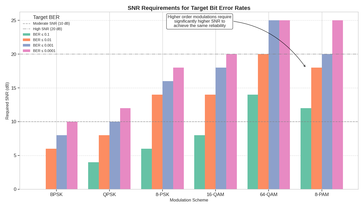
SNR Requirements for Target BER

Different applications have different BER requirements. Let’s visualize the minimum SNR required for each modulation scheme to achieve various target BERs.

# Define target BER values
target_bers = [1e-1, 1e-2, 1e-3, 1e-4]

# Find minimum SNR required for each modulation to achieve each target BER
snr_requirements: dict[str, list[float]] = {name: [] for name, _, _ in modulation_schemes}

for name, __, ___ in modulation_schemes:
    for target in target_bers:
        # Find the first SNR that achieves the target BER or better
        ber_array = np.array(ber_results[name])
        indices = np.where(ber_array <= target)[0]

        if len(indices) > 0:
            min_snr = snr_db_range[indices[0]]
        else:
            # If target can't be achieved, use a high value
            min_snr = snr_db_range[-1] + 5

        snr_requirements[name].append(min_snr)

# Create grouped bar chart
fig, ax = plt.subplots(figsize=(14, 8))

x = np.arange(len(scheme_names))
width = 0.2
multiplier = 0

for i, target in enumerate(target_bers):
    offset = width * multiplier
    rects = ax.bar(x + offset, [snr_requirements[name][i] for name in scheme_names], width, label=f"BER ≤ {target}", color=accent_colors[i])
    multiplier += 1

# Add horizontal lines for key SNR benchmarks
ax.axhline(y=10, color="gray", linestyle="--", alpha=0.7, label="Moderate SNR (10 dB)")
ax.axhline(y=20, color="gray", linestyle="-.", alpha=0.7, label="High SNR (20 dB)")

# Format the plot
ax.set_ylabel("Required SNR (dB)", fontsize=12)
ax.set_xlabel("Modulation Scheme", fontsize=12)
ax.set_title("SNR Requirements for Target Bit Error Rates", fontsize=16, fontweight="bold")
ax.set_xticks(x + width * (len(target_bers) - 1) / 2)
ax.set_xticklabels(scheme_names)
ax.legend(title="Target BER", loc="upper left", fontsize=10)
ax.grid(True, axis="y", linestyle="--", alpha=0.7)

# Add annotation to explain practical implications
plt.annotate(
    "Higher order modulations require\nsignificantly higher SNR to\nachieve the same reliability", xy=(5, 18), xytext=(3, 24), arrowprops=dict(arrowstyle="->", connectionstyle="arc3,rad=-0.3"), bbox=dict(boxstyle="round,pad=0.3", fc="white", ec="black", alpha=0.8), fontsize=12, ha="center"
)

plt.tight_layout()

Spectral Efficiency vs. Power Efficiency Tradeoff

The key tradeoff in modulation design is between spectral efficiency and power efficiency. Let’s visualize this tradeoff to help understand how to select the right modulation for different scenarios.

# Estimate power efficiency by finding SNR required for BER = 1e-3
power_efficiency = []
for name, ____, _____ in modulation_schemes:
    req_snr = snr_requirements[name][2]  # Index 2 corresponds to BER=1e-3 in our target_bers list
    # Convert from dB to linear for calculating efficiency
    power_efficiency.append(1 / (10 ** (req_snr / 10)))

# Create scatter plot
plt.figure(figsize=(12, 8))
plt.scatter(spectral_efficiency, power_efficiency, s=200, c=accent_colors[: len(spectral_efficiency)], alpha=0.7)

# Add labels for each point
for i, name in enumerate(scheme_names):
    plt.annotate(name, (spectral_efficiency[i], power_efficiency[i]), xytext=(5, 5), textcoords="offset points", fontsize=12, fontweight="bold")

# Add connecting line to show trend
plt.plot(spectral_efficiency, power_efficiency, "k--", alpha=0.5)

# Format the plot
plt.xlabel("Spectral Efficiency (bits/symbol)", fontsize=14)
plt.ylabel("Power Efficiency (normalized)", fontsize=14)
plt.title("Modulation Scheme Tradeoff: Spectral vs. Power Efficiency", fontsize=16, fontweight="bold")
plt.grid(True, linestyle="--", alpha=0.7)

# Add quadrant labels to help with scheme selection
plt.text(1.5, 0.9 * max(power_efficiency), "Higher Power Efficiency\nLower Spectral Efficiency", fontsize=12, ha="center", va="center", bbox=dict(boxstyle="round,pad=0.3", fc="lightgray", ec="gray", alpha=0.7))

plt.text(5, 0.2 * max(power_efficiency), "Higher Spectral Efficiency\nLower Power Efficiency", fontsize=12, ha="center", va="center", bbox=dict(boxstyle="round,pad=0.3", fc="lightgray", ec="gray", alpha=0.7))

# Add application examples
plt.annotate("Satellite/Deep Space\nCommunications", xy=(1, power_efficiency[0]), xytext=(1, power_efficiency[0] * 1.2), arrowprops=dict(arrowstyle="->", connectionstyle="arc3,rad=0.3"), bbox=dict(boxstyle="round,pad=0.3", fc="#e6f7ff", ec="blue", alpha=0.8), fontsize=10, ha="center")

plt.annotate("Mobile Communications", xy=(2, power_efficiency[1]), xytext=(2.5, power_efficiency[1] * 1.2), arrowprops=dict(arrowstyle="->", connectionstyle="arc3,rad=0.3"), bbox=dict(boxstyle="round,pad=0.3", fc="#e6f7ff", ec="blue", alpha=0.8), fontsize=10, ha="center")

plt.annotate("Wi-Fi, Fiber Optics\nData Centers", xy=(6, power_efficiency[4]), xytext=(4.5, power_efficiency[4] * 1.5), arrowprops=dict(arrowstyle="->", connectionstyle="arc3,rad=-0.3"), bbox=dict(boxstyle="round,pad=0.3", fc="#e6f7ff", ec="blue", alpha=0.8), fontsize=10, ha="center")

plt.tight_layout()

Dynamic Modulation Selection Based on Channel Conditions

In adaptive modulation systems, the modulation scheme changes based on channel conditions. Let’s implement and visualize a simple adaptive modulation scheme.

class AdaptiveModulation:
    """A simple adaptive modulation scheme that selects the modulation based on SNR."""

    def __init__(self):
        # Define modulation schemes with their SNR thresholds for BER ≤ 1e-3
        self.schemes = [
            {"name": "BPSK", "module": Modem(BPSKModulator(), BPSKDemodulator(), soft_output=False), "bits_per_symbol": 1, "min_snr": 0, "max_snr": 7, "color": accent_colors[0]},
            {"name": "QPSK", "module": Modem(QPSKModulator(), QPSKDemodulator(), soft_output=False), "bits_per_symbol": 2, "min_snr": 7, "max_snr": 12, "color": accent_colors[1]},
            {"name": "8-PSK", "module": Modem(PSKModulator(order=8), PSKDemodulator(order=8), soft_output=False), "bits_per_symbol": 3, "min_snr": 12, "max_snr": 17, "color": accent_colors[2]},
            {"name": "16-QAM", "module": Modem(QAMModulator(order=16), QAMDemodulator(order=16), soft_output=False), "bits_per_symbol": 4, "min_snr": 17, "max_snr": 25, "color": accent_colors[3]},
            {"name": "64-QAM", "module": Modem(QAMModulator(order=64), QAMDemodulator(order=64), soft_output=False), "bits_per_symbol": 6, "min_snr": 25, "max_snr": 100, "color": accent_colors[4]},
        ]

    def select_scheme(self, snr_db):
        """Select the appropriate modulation scheme based on SNR."""
        for scheme in self.schemes:
            if scheme["min_snr"] <= snr_db < scheme["max_snr"]:
                return scheme
        # Default to the highest order scheme for very high SNR
        return self.schemes[-1]

    def get_spectral_efficiency(self, snr_db):
        """Get spectral efficiency for the selected scheme at given SNR."""
        scheme = self.select_scheme(snr_db)
        return scheme["bits_per_symbol"]


# Create an instance of the adaptive modulation system
adaptive_mod = AdaptiveModulation()

# Visualize the adaptive modulation strategy
plt.figure(figsize=(14, 8))

# Plot SNR ranges for each modulation scheme
snr_range = np.arange(0, 30, 0.1)
spectral_eff = [adaptive_mod.get_spectral_efficiency(snr) for snr in snr_range]

plt.plot(snr_range, spectral_eff, "k-", linewidth=3, label="Adaptive Selection")

# Add colored regions for each modulation scheme
for scheme in adaptive_mod.schemes:
    plt.axvspan(scheme["min_snr"], scheme["max_snr"], alpha=0.2, color=scheme["color"], label=f"{scheme['name']} ({scheme['bits_per_symbol']} bits/symbol)")

# Format the plot
plt.xlabel("Channel SNR (dB)", fontsize=14)
plt.ylabel("Spectral Efficiency (bits/symbol)", fontsize=14)
plt.title("Adaptive Modulation: Dynamic Scheme Selection Based on Channel Conditions", fontsize=16, fontweight="bold")
plt.grid(True, linestyle="--", alpha=0.7)
plt.legend(loc="upper left", fontsize=12)

# Add explanatory annotations
plt.annotate("Adaptive modulation increases spectral efficiency\nwhen channel conditions are favorable", xy=(22, 5), xytext=(15, 3), arrowprops=dict(arrowstyle="->", connectionstyle="arc3,rad=0.3"), bbox=dict(boxstyle="round,pad=0.3", fc="white", ec="black", alpha=0.8), fontsize=12, ha="center")

plt.annotate("Falls back to robust schemes\nwhen channel conditions degrade", xy=(5, 1.2), xytext=(10, 2), arrowprops=dict(arrowstyle="->", connectionstyle="arc3,rad=-0.3"), bbox=dict(boxstyle="round,pad=0.3", fc="white", ec="black", alpha=0.8), fontsize=12, ha="center")

plt.tight_layout()

Simulating a Time-Varying Channel with Adaptive Modulation

Let’s simulate a time-varying channel and show how adaptive modulation responds.

# Simulate a time-varying channel with SNR fluctuations
time_steps = 100
time = np.arange(time_steps)

# Create a realistic SNR pattern with:
# 1. A slow trend component (e.g., user moving closer/further from the base station)
# 2. Fast fading component (e.g., multipath fading)
# 3. Random noise component (e.g., interference)

slow_trend = 15 + 10 * np.sin(2 * np.pi * time / time_steps)  # 5-25 dB range
fast_fading = 3 * np.sin(2 * np.pi * time / 10)  # ±3 dB fading
random_component = np.random.normal(0, 1, time_steps)  # Random fluctuations

channel_snr = slow_trend + fast_fading + random_component
channel_snr = np.clip(channel_snr, 0, 30)  # Ensure SNR stays in reasonable range

# Determine modulation scheme at each time step
selected_schemes = []
throughput = []
bit_error_rates = []

for snr in channel_snr:
    # Select scheme based on current SNR
    scheme = adaptive_mod.select_scheme(snr)  # This returns a dict, not a Modem
    selected_schemes.append(scheme)

    # Calculate throughput (normalized by max possible)
    throughput.append(scheme["bits_per_symbol"] / 6)  # Normalize by max (64-QAM = 6 bits)

    # Estimate BER for this scheme at this SNR
    # Use simple approximations for demonstration
    if scheme["name"] == "BPSK":
        ber = q_function(np.sqrt(2 * 10 ** (snr / 10)))
    elif scheme["name"] == "QPSK":
        ber = q_function(np.sqrt(10 ** (snr / 10)))
    elif scheme["name"] == "8-PSK":
        ber = 2 * q_function(np.sqrt(2 * 10 ** (snr / 10)) * np.sin(np.pi / 8))
    elif scheme["name"] == "16-QAM":
        ber = 0.75 * q_function(np.sqrt(0.2 * 10 ** (snr / 10)))
    else:  # 64-QAM
        ber = 0.83 * q_function(np.sqrt(0.1 * 10 ** (snr / 10)))

    bit_error_rates.append(min(ber, 1))  # Cap at 1 for display purposes

# Visualize the results
fig = plt.figure(figsize=(14, 10))
gs = GridSpec(3, 1, figure=fig, height_ratios=[1, 1, 1], hspace=0.4)  # Increase hspace for better separation

# Plot 1: Channel SNR variation over time
ax1 = fig.add_subplot(gs[0])
ax1.plot(time, channel_snr, "b-", linewidth=2)
ax1.set_xlabel("Time", fontsize=12)
ax1.set_ylabel("Channel SNR (dB)", fontsize=12)
ax1.set_title("Time-Varying Channel Conditions", fontsize=14, fontweight="bold")
ax1.grid(True, linestyle="--", alpha=0.7)

# Add threshold lines for modulation switches
for scheme in adaptive_mod.schemes[:-1]:
    ax1.axhline(y=scheme["max_snr"], color="gray", linestyle="--", alpha=0.5)
    ax1.text(time[-1] + 1, scheme["max_snr"], f"Switch to {adaptive_mod.schemes[adaptive_mod.schemes.index(scheme) + 1]['name']}", fontsize=8, va="center")

# Plot 2: Selected modulation scheme over time
ax2 = fig.add_subplot(gs[1])
# Get the indices of the schemes instead of assigning the schemes directly
scheme_indices = [adaptive_mod.schemes.index(s) for s in selected_schemes]
scheme_colors = [s["color"] for s in selected_schemes]  # Direct color values, not strings
ax2.scatter(time, scheme_indices, c=scheme_colors, s=50, alpha=0.7)

# Connect the dots
ax2.plot(time, scheme_indices, "k-", alpha=0.3)

# Set custom y-ticks for modulation schemes
ax2.set_yticks(range(len(adaptive_mod.schemes)))
ax2.set_yticklabels([f"{s['name']} ({s['bits_per_symbol']} bits)" for s in adaptive_mod.schemes])
ax2.set_xlabel("Time", fontsize=12)
ax2.set_ylabel("Selected Modulation", fontsize=12)
ax2.set_title("Adaptive Modulation Response to Channel Variations", fontsize=14, fontweight="bold")
ax2.grid(True, linestyle="--", alpha=0.7)

# Plot 3: Throughput and estimated BER over time
ax3 = fig.add_subplot(gs[2])

# Plot throughput
(line1,) = ax3.plot(time, throughput, "g-", linewidth=2, label="Normalized Throughput")
ax3.set_xlabel("Time", fontsize=12)
ax3.set_ylabel("Normalized Throughput", fontsize=12, color="g")
ax3.tick_params(axis="y", labelcolor="g")
ax3.set_ylim(0, 1.1)

# Add second y-axis for BER
ax3b = ax3.twinx()
(line2,) = ax3b.semilogy(time, bit_error_rates, "r-", linewidth=2, label="Bit Error Rate")
ax3b.set_ylabel("Bit Error Rate (log scale)", fontsize=12, color="r")
ax3b.tick_params(axis="y", labelcolor="r")
ax3b.set_ylim(1e-6, 1)

# Add combined legend
lines = [line1, line2]
ax3.legend(lines, [str(line.get_label()) for line in lines], loc="upper right")
ax3.set_title("System Performance with Adaptive Modulation", fontsize=14, fontweight="bold")
ax3.grid(True, linestyle="--", alpha=0.7)

# Add annotation to highlight adaptive trade-off
lower_throughput_phase = 40  # Time step with lower throughput/higher reliability
higher_throughput_phase = 75  # Time step with higher throughput/lower reliability

ax3.annotate("Consistent BER despite\nchannel variations", xy=(time_steps / 2, 0.5), xytext=(time_steps / 2 - 15, 0.7), arrowprops=dict(arrowstyle="->", connectionstyle="arc3,rad=0.3"), bbox=dict(boxstyle="round,pad=0.3", fc="white", ec="black", alpha=0.8), fontsize=10, ha="center")

plt.suptitle("Adaptive Modulation in a Time-Varying Channel Environment", fontsize=16, fontweight="bold", y=0.98)
plt.subplots_adjust(left=0.08, right=0.92, bottom=0.08, top=0.92)

Conclusion and Key Takeaways

Through this example, we’ve examined various digital modulation schemes available in Kaira:

• Basic modulation schemes: BPSK, QPSK, PSK, QAM, and PAM with different orders

• Constellation diagrams: Visual representation of symbol mapping

• BER performance: How different schemes perform under noise

• Spectral vs. power efficiency tradeoff: Higher order modulations offer better spectral efficiency but require higher SNR

• Adaptive modulation: Dynamically selecting modulation based on channel conditions

For practical applications:

1. Choose lower-order modulations (BPSK, QPSK) for reliability in challenging channels

2. Choose higher-order modulations (16-QAM, 64-QAM) for high data rates in good channels

3. Consider adaptive modulation to optimize performance as channel conditions change

4. The choice of modulation scheme significantly impacts both system performance and complexity

Kaira provides a flexible framework for implementing and experimenting with these various modulation schemes, allowing researchers and engineers to develop and test advanced communication systems.