Digital Binary Channels in Kaira

This example demonstrates the usage of binary channel models in Kaira. Binary channels are fundamental in digital communications as they represent the transmission of binary data (0s and 1s) through a noisy medium.

We’ll explore the three main binary channel models: 1. Binary Symmetric Channel (BSC) 2. Binary Erasure Channel (BEC) 3. Binary Z-Channel

Imports and Setup

We start by importing the necessary modules and setting up the environment.

import matplotlib.pyplot as plt
import numpy as np
import seaborn as sns
import torch

from kaira.channels import BinaryErasureChannel, BinarySymmetricChannel, BinaryZChannel

# Set random seed for reproducibility
torch.manual_seed(42)
np.random.seed(42)

Generate Binary Data

Let’s generate a random binary sequence to transmit through our channels.

# Generate 1000 random binary values (0 or 1)
num_bits = 1000
binary_data = torch.randint(0, 2, (1, num_bits)).float()

print(f"Generated {num_bits} random bits")
print(f"First 20 bits: {binary_data[0, :20].int().tolist()}")

Generated 1000 random bits
First 20 bits: [0, 1, 0, 0, 0, 1, 0, 0, 0, 1, 0, 0, 0, 0, 1, 0, 1, 1, 1, 0]

Binary Symmetric Channel (BSC)

The BSC flips bits with probability p. Both 0→1 and 1→0 transitions occur with the same probability.

# Create BSC with different error probabilities
error_probs = [0.01, 0.05, 0.1, 0.2, 0.5]
bsc_outputs = []

for p in error_probs:
    # Create the channel
    bsc = BinarySymmetricChannel(crossover_prob=p)

    # Pass data through the channel
    with torch.no_grad():
        output = bsc(binary_data)

    # Calculate bit error rate
    errors = (output != binary_data).sum().item()
    error_rate = errors / num_bits

    bsc_outputs.append((p, output, error_rate))
    print(f"BSC (p={p}): Errors: {errors}/{num_bits}, Error rate: {error_rate:.4f}")

BSC (p=0.01): Errors: 7/1000, Error rate: 0.0070
BSC (p=0.05): Errors: 42/1000, Error rate: 0.0420
BSC (p=0.1): Errors: 97/1000, Error rate: 0.0970
BSC (p=0.2): Errors: 198/1000, Error rate: 0.1980
BSC (p=0.5): Errors: 486/1000, Error rate: 0.4860

Binary Erasure Channel (BEC)

The BEC erases bits with probability p, replacing them with a special “erasure” symbol (here represented by -1).

# Create BEC with different erasure probabilities
erasure_probs = [0.01, 0.05, 0.1, 0.2, 0.5]
bec_outputs = []

for p in erasure_probs:
    # Create the channel
    bec = BinaryErasureChannel(erasure_prob=p)

    # Pass data through the channel
    with torch.no_grad():
        output = bec(binary_data)

    # Count erasures
    erasures = (output == -1).sum().item()
    erasure_rate = erasures / num_bits

    bec_outputs.append((p, output, erasure_rate))
    print(f"BEC (p={p}): Erasures: {erasures}/{num_bits}, Erasure rate: {erasure_rate:.4f}")

BEC (p=0.01): Erasures: 11/1000, Erasure rate: 0.0110
BEC (p=0.05): Erasures: 54/1000, Erasure rate: 0.0540
BEC (p=0.1): Erasures: 98/1000, Erasure rate: 0.0980
BEC (p=0.2): Erasures: 199/1000, Erasure rate: 0.1990
BEC (p=0.5): Erasures: 513/1000, Erasure rate: 0.5130

Binary Z-Channel

The Z-Channel has asymmetric error probabilities. Only 1→0 transitions occur with probability p.

# Create Z-Channel with different error probabilities
z_error_probs = [0.01, 0.05, 0.1, 0.2, 0.5]
z_outputs = []

for p in z_error_probs:
    # Create the channel
    z_channel = BinaryZChannel(error_prob=p)

    # Pass data through the channel
    with torch.no_grad():
        output = z_channel(binary_data)

    # Calculate errors (only 1→0 flips can occur)
    original_ones = binary_data == 1
    errors = ((output != binary_data) & original_ones).sum().item()
    ones_count = original_ones.sum().item()
    error_rate = errors / ones_count if ones_count > 0 else 0

    z_outputs.append((p, output, error_rate))
    print(f"Z-Channel (p={p}): 1→0 Errors: {errors}/{ones_count}, Error rate: {error_rate:.4f}")

Z-Channel (p=0.01): 1→0 Errors: 4/510, Error rate: 0.0078
Z-Channel (p=0.05): 1→0 Errors: 29/510, Error rate: 0.0569
Z-Channel (p=0.1): 1→0 Errors: 50/510, Error rate: 0.0980
Z-Channel (p=0.2): 1→0 Errors: 98/510, Error rate: 0.1922
Z-Channel (p=0.5): 1→0 Errors: 255/510, Error rate: 0.5000

Visualizing Channel Effects

Let’s visualize a small segment of the data to see how each channel affects the binary transmission.

# Take a small segment of the data for visualization
segment_start = 0
segment_length = 50
segment_data = binary_data[0, segment_start : segment_start + segment_length].numpy()


# Create a function to visualize binary data
def plot_binary_data(ax, data, title, y_pos, erasures=None):
    """Plot binary data with optional erasure markers."""
    # Plot 0s and 1s
    ax.scatter(np.arange(len(data)), [y_pos] * len(data), c=["blue" if b == 1 else "red" for b in data], marker="o", s=50)

    # Mark erasures if provided
    if erasures is not None:
        erasure_indices = np.where(erasures)[0]
        if len(erasure_indices) > 0:
            ax.scatter(erasure_indices, [y_pos] * len(erasure_indices), facecolors="none", edgecolors="black", marker="o", s=80, linewidth=2)

    ax.set_ylabel(title)
    ax.set_ylim(y_pos - 0.5, y_pos + 0.5)
    ax.set_yticks([])

    return ax


# Create visualization
fig, axes = plt.subplots(7, 1, figsize=(12, 10), sharex=True)
plt.subplots_adjust(hspace=0.3)

# Plot original data
plot_binary_data(axes[0], segment_data, "Original", 0)

# Plot BSC output (high error probability for visibility)
bsc_p = 0.2
bsc = BinarySymmetricChannel(crossover_prob=bsc_p)
with torch.no_grad():
    bsc_output = bsc(binary_data[:, segment_start : segment_start + segment_length]).numpy()[0]
plot_binary_data(axes[1], bsc_output, f"BSC (p={bsc_p})", 0)

# Plot BEC output (high erasure probability for visibility)
bec_p = 0.2
bec = BinaryErasureChannel(erasure_prob=bec_p)
with torch.no_grad():
    bec_output = bec(binary_data[:, segment_start : segment_start + segment_length]).numpy()[0]
bec_erasures = bec_output == -1
bec_output = np.where(bec_erasures, 0.5, bec_output)  # Replace erasures with 0.5 for visualization
plot_binary_data(axes[2], bec_output, f"BEC (p={bec_p})", 0, erasures=bec_erasures)

# Plot Z-Channel output (high error probability for visibility)
z_p = 0.5  # Higher for visibility since it only affects 1→0 transitions
z_channel = BinaryZChannel(error_prob=z_p)
with torch.no_grad():
    z_output = z_channel(binary_data[:, segment_start : segment_start + segment_length]).numpy()[0]
plot_binary_data(axes[3], z_output, f"Z-Channel (p={z_p})", 0)

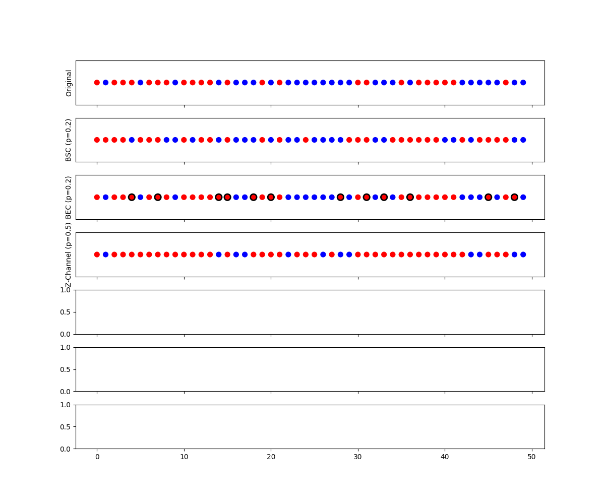
<Axes: ylabel='Z-Channel (p=0.5)'>

Comparing Error Rates Across Channels

Now let’s compare the theoretical vs. observed error rates for each channel type.

# Add horizontal lines for bit positions
for ax in axes[:4]:
    ax.set_xlim(-1, segment_length)
    ax.set_xticks(np.arange(0, segment_length, 5))
    ax.grid(True, axis="x", linestyle="--", alpha=0.7)

axes[3].set_xlabel("Bit Position")

# Plot error rates for BSC
ax = axes[4]
theoretical_bsc = error_probs  # Theoretical error rate equals p
observed_bsc = [err_rate for _, _, err_rate in bsc_outputs]
ax.plot(error_probs, theoretical_bsc, "b-", label="Theoretical")
ax.plot(error_probs, observed_bsc, "bo--", label="Observed")
ax.set_ylabel("BSC Error Rate")
ax.grid(True)
ax.legend()

# Plot erasure rates for BEC
ax = axes[5]
theoretical_bec = erasure_probs  # Theoretical erasure rate equals p
observed_bec = [erasure_rate for _, _, erasure_rate in bec_outputs]
ax.plot(erasure_probs, theoretical_bec, "g-", label="Theoretical")
ax.plot(erasure_probs, observed_bec, "go--", label="Observed")
ax.set_ylabel("BEC Erasure Rate")
ax.grid(True)
ax.legend()

# Plot error rates for Z-Channel
ax = axes[6]
# Theoretical error rate for Z-channel is p * P(1), where P(1) is probability of input being 1
p_one = (binary_data == 1).sum().item() / num_bits
theoretical_z = [p * p_one for p in z_error_probs]
observed_z = [err_rate * p_one for _, _, err_rate in z_outputs]
ax.plot(z_error_probs, theoretical_z, "r-", label="Theoretical")
ax.plot(z_error_probs, observed_z, "ro--", label="Observed")
ax.set_xlabel("Channel Parameter (p)")
ax.set_ylabel("Z-Channel Error Rate")
ax.grid(True)
ax.legend()

plt.tight_layout()
plt.show()

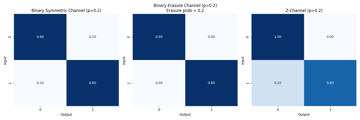
Channel Transition Matrices

Visualize the transition matrices for each channel type.

def plot_transition_matrix(ax, matrix, title):
    """Plot a channel transition matrix."""
    sns.heatmap(matrix, annot=True, fmt=".2f", cmap="Blues", cbar=False, ax=ax)
    ax.set_title(title)
    ax.set_xlabel("Output")
    ax.set_ylabel("Input")
    ax.set_xticks([0.5, 1.5])
    ax.set_xticklabels(["0", "1"])
    ax.set_yticks([0.5, 1.5])
    ax.set_yticklabels(["0", "1"])
    return ax


# Create a figure with 3 subplots
fig, axes = plt.subplots(1, 3, figsize=(15, 5))

# BSC transition matrix [p=0.2]
p_bsc = 0.2
bsc_matrix = np.array([[1 - p_bsc, p_bsc], [p_bsc, 1 - p_bsc]])
plot_transition_matrix(axes[0], bsc_matrix, f"Binary Symmetric Channel (p={p_bsc})")

# BEC transition matrix [p=0.2]
p_bec = 0.2
# For BEC, we use -1 to represent erasure, but for visualization we'll use a 3x2 matrix
bec_matrix = np.array([[1 - p_bec, 0], [0, 1 - p_bec]])
plot_transition_matrix(axes[1], bec_matrix, f"Binary Erasure Channel (p={p_bec})\nErasure prob = {p_bec}")

# Z-Channel transition matrix [p=0.2]
p_z = 0.2
z_matrix = np.array([[1, 0], [p_z, 1 - p_z]])
plot_transition_matrix(axes[2], z_matrix, f"Z-Channel (p={p_z})")

plt.tight_layout()
plt.show()

Conclusion

This example demonstrated the use of different binary channel models in Kaira:

• The Binary Symmetric Channel randomly flips bits with probability p, affecting both 0→1 and 1→0 transitions equally.

• The Binary Erasure Channel randomly erases bits with probability p, converting them to an erasure symbol (often useful in coding theory).

• The Z-Channel has asymmetric error probability, where only 1→0 transitions occur with probability p (common in some physical systems).

These binary channels serve as building blocks for more complex digital communication systems and are fundamental in information theory for analyzing capacity and error rates.