Quadrature Amplitude Modulation (QAM)

This example demonstrates the usage of Quadrature Amplitude Modulation (QAM) in the Kaira library. We’ll explore different QAM orders (4-QAM, 16-QAM, 64-QAM) and analyze their performance characteristics.

import matplotlib.pyplot as plt

Imports and Setup

import numpy as np
import torch

from kaira.channels import AWGNChannel
from kaira.metrics.signal import BER
from kaira.modulations import QAMDemodulator, QAMModulator
from kaira.modulations.utils import plot_constellation
from kaira.utils import snr_to_noise_power

# Set random seed for reproducibility
torch.manual_seed(42)
np.random.seed(42)

Create QAM Modulators with Different Orders

qam_orders: list[int] = [4, 16, 64]
n_symbols = 1000

modulators: dict[int, QAMModulator] = {order: QAMModulator(order=order) for order in qam_orders}  # type: ignore
demodulators: dict[int, QAMDemodulator] = {order: QAMDemodulator(order=order) for order in qam_orders}  # type: ignore

# Generate random bits for each QAM order
bits_per_symbol = {4: 2, 16: 4, 64: 6}  # 4-QAM (same as QPSK)  # 16-QAM  # 64-QAM

input_bits = {}
modulated_symbols = {}
for order in qam_orders:
    n_bits = bits_per_symbol[order] * n_symbols
    input_bits[order] = torch.randint(0, 2, (1, n_bits))
    modulated_symbols[order] = modulators[order](input_bits[order])

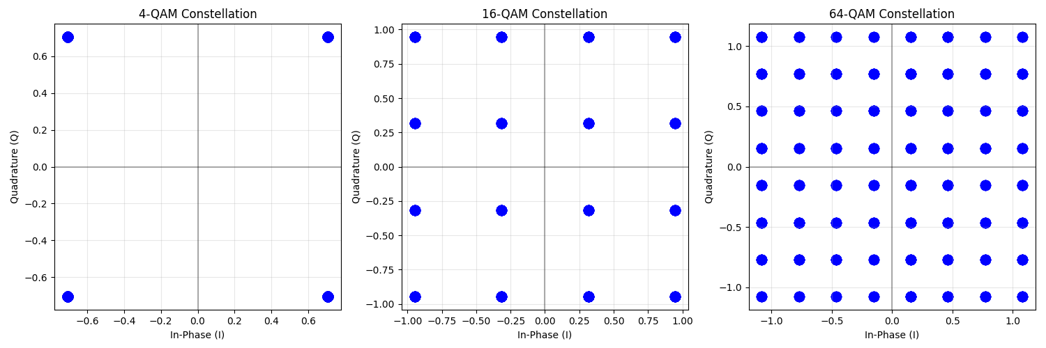
Plot Constellation Diagrams

fig, axs = plt.subplots(1, 3, figsize=(15, 5))
for i, order in enumerate(qam_orders):
    plot_constellation(modulated_symbols[order].flatten(), title=f"{order}-QAM Constellation", marker="o", ax=axs[i])
    axs[i].grid(True)
plt.tight_layout()
plt.show()

Simulate Transmission over AWGN Channel

snr_db_range = np.arange(0, 31, 2)
ber_results: dict[int, list[float]] = {order: [] for order in qam_orders}

# Initialize BER metric
ber_metric = BER()

for snr_db in snr_db_range:
    noise_power = snr_to_noise_power(1.0, snr_db)
    channel = AWGNChannel(avg_noise_power=noise_power)

    for order in qam_orders:
        # Transmit through channel
        received = channel(modulated_symbols[order])

        # Demodulate
        demod_bits = demodulators[order](received)

        # Calculate BER
        ber = ber_metric(demod_bits, input_bits[order]).item()
        ber_results[order].append(ber)

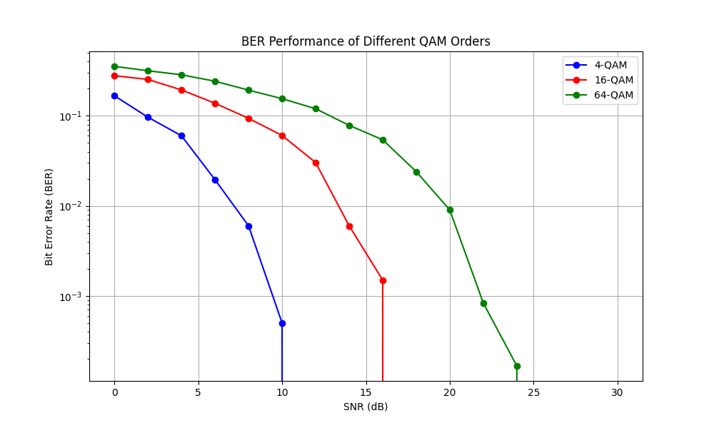
Plot BER vs SNR Performance

plt.figure(figsize=(10, 6))

colors = ["b", "r", "g"]
for order, color in zip(qam_orders, colors):
    plt.semilogy(snr_db_range, ber_results[order], f"{color}o-", label=f"{order}-QAM")

plt.grid(True)
plt.xlabel("SNR (dB)")
plt.ylabel("Bit Error Rate (BER)")
plt.title("BER Performance of Different QAM Orders")
plt.legend()
plt.show()

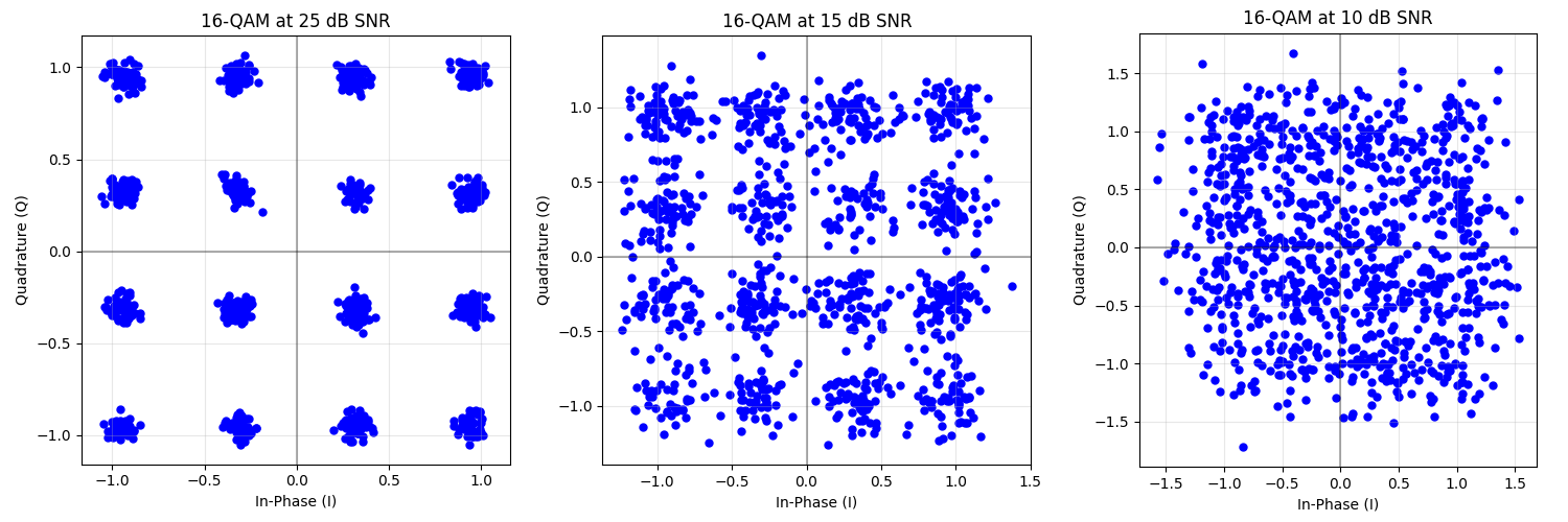
Visualize Effect of Noise on 16-QAM

test_snr_db = [25, 15, 10]
n_test_symbols = 1000
qam16_mod = modulators[16]

fig, axs = plt.subplots(1, 3, figsize=(15, 5))

# Generate random 16-QAM symbols
test_bits = torch.randint(0, 2, (1, 4 * n_test_symbols))  # 4 bits per symbol for 16-QAM
qam16_symbols = qam16_mod(test_bits)

for i, snr_db in enumerate(test_snr_db):
    noise_power = snr_to_noise_power(1.0, snr_db)
    channel = AWGNChannel(avg_noise_power=noise_power)

    # Pass through noisy channel
    received_symbols = channel(qam16_symbols)

    plot_constellation(received_symbols.flatten(), title=f"16-QAM at {snr_db} dB SNR", marker=".", ax=axs[i])
    axs[i].grid(True)

plt.tight_layout()
plt.show()

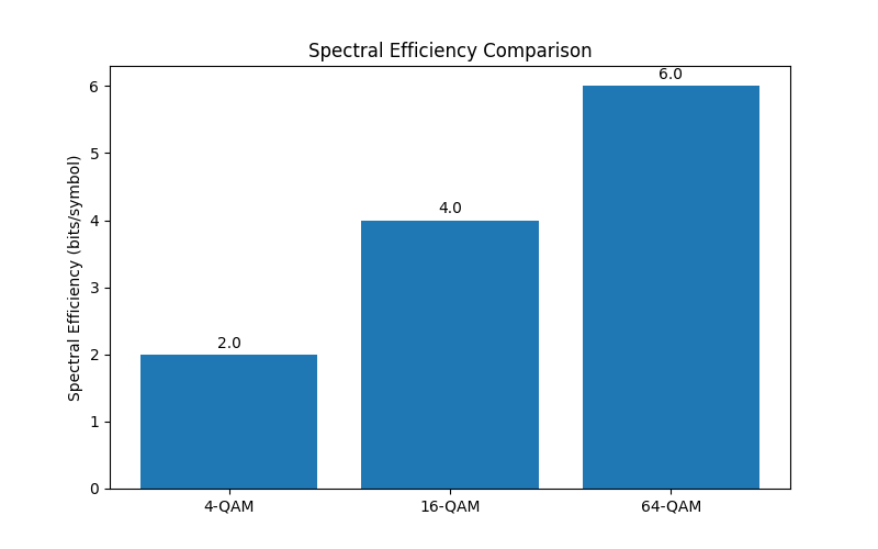
Spectral Efficiency Comparison

plt.figure(figsize=(8, 5))

# Calculate spectral efficiency (bits/symbol)
spectral_efficiency = [np.log2(order) for order in qam_orders]

plt.bar(range(len(qam_orders)), spectral_efficiency)
plt.xticks(range(len(qam_orders)), [f"{order}-QAM" for order in qam_orders])
plt.ylabel("Spectral Efficiency (bits/symbol)")
plt.title("Spectral Efficiency Comparison")

for i, v in enumerate(spectral_efficiency):
    plt.text(i, v + 0.1, f"{v:.1f}", ha="center")

plt.show()

Conclusion

This example demonstrated:

1. Implementation of different QAM orders using Kaira

2. Constellation visualization for 4-QAM, 16-QAM, and 64-QAM

3. BER performance analysis across different SNR levels

4. Effect of noise on constellation diagrams

5. Spectral efficiency comparison

Key observations:

• Higher-order QAM schemes offer increased spectral efficiency

• As QAM order increases, more SNR is required for reliable communication

• 64-QAM requires approximately 10dB more SNR than 4-QAM for the same BER

• Constellation points become more difficult to distinguish at lower SNR

• There’s a clear trade-off between spectral efficiency and noise sensitivity