Finite Field Algebra for FEC Codes

This example demonstrates the algebraic foundations of forward error correction (FEC) codes using the binary polynomial and finite field utilities in the kaira.models.fec.algebra module. These algebraic structures are essential for advanced codes like BCH, Reed-Solomon, and other algebraic error correction codes.

import matplotlib.pyplot as plt
import numpy as np
import torch

from kaira.models.fec.algebra import BinaryPolynomial, FiniteBifield

Setting up

First, we set a random seed to ensure reproducibility of results.

torch.manual_seed(42)
np.random.seed(42)

Binary Polynomials

Binary polynomials are polynomials with coefficients from the field GF(2), which contains only two elements: 0 and 1. They are represented using their integer values, where each bit position corresponds to a coefficient.

# Create some binary polynomials
p1 = BinaryPolynomial(0b1011)  # x³ + x + 1
p2 = BinaryPolynomial(0b110)  # x² + x
p3 = BinaryPolynomial(0b1)  # 1
p4 = BinaryPolynomial(0b0)  # 0 (zero polynomial)

print(f"p1 = {p1} (binary: {bin(p1.value)})")
print(f"p2 = {p2} (binary: {bin(p2.value)})")
print(f"p3 = {p3} (binary: {bin(p3.value)})")
print(f"p4 = {p4} (binary: {bin(p4.value)})")

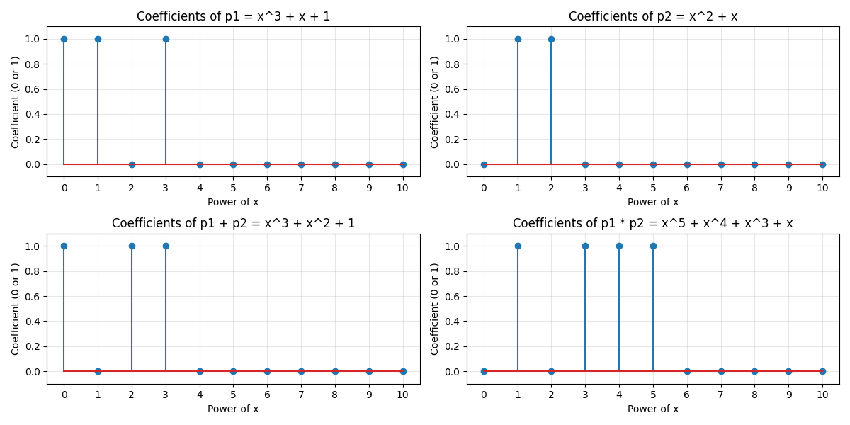
p1 = x^3 + x + 1 (binary: 0b1011)
p2 = x^2 + x (binary: 0b110)
p3 = 1 (binary: 0b1)
p4 = 0 (binary: 0b0)

Basic Operations

Binary polynomials support various operations like addition, multiplication, and modular arithmetic. In GF(2), addition is implemented using XOR, which means 1 + 1 = 0.

# Addition (XOR operation in GF(2))
sum_poly = BinaryPolynomial(p1.value ^ p2.value)
print(f"p1 + p2 = {sum_poly} (binary: {bin(sum_poly.value)})")

# Multiplication
product = p1 * p2
print(f"p1 * p2 = {product} (binary: {bin(product.value)})")

# Division and modular arithmetic
quotient = p1.div(p2)
remainder = p1 % p2
print(f"p1 ÷ p2 = {quotient} with remainder {remainder}")

# Greatest Common Divisor (GCD)
gcd = p1.gcd(p2)
print(f"GCD(p1, p2) = {gcd}")

p1 + p2 = x^3 + x^2 + 1 (binary: 0b1101)
p1 * p2 = x^5 + x^4 + x^3 + x (binary: 0b111010)
p1 ÷ p2 = x + 1 with remainder 1
GCD(p1, p2) = 1

Polynomial Evaluation

We can evaluate polynomials at specific points, which is essential for error correction algorithms.

# Evaluate at some points
x_values = [0, 1, 2, 3, 4]
evaluations = [p1.evaluate(x) for x in x_values]

print("Evaluating p1 at different points:")
for x, y in zip(x_values, evaluations):
    print(f"p1({x}) = {y}")

Evaluating p1 at different points:
p1(0) = 1
p1(1) = 1
p1(2) = 11
p1(3) = 25
p1(4) = 69

Visualizing Polynomial Operations

Let’s visualize our binary polynomials and some operations.

# Function to convert polynomial to coefficient array for plotting
def poly_to_coeff_array(poly, max_degree=10):
    """Convert a binary polynomial to a coefficient array for plotting."""
    coeffs = np.zeros(max_degree + 1)
    for i, c in enumerate(poly.to_coefficient_list()):
        if i <= max_degree:
            coeffs[i] = c
    return coeffs


# Plot the coefficients of the polynomials
max_degree = 10
plt.figure(figsize=(12, 6))

plt.subplot(2, 2, 1)
coeffs = poly_to_coeff_array(p1, max_degree)
plt.stem(np.arange(len(coeffs)), coeffs)
plt.title(f"Coefficients of p1 = {p1}")
plt.xlabel("Power of x")
plt.ylabel("Coefficient (0 or 1)")
plt.ylim(-0.1, 1.1)
plt.xticks(np.arange(max_degree + 1))
plt.grid(True, alpha=0.3)

plt.subplot(2, 2, 2)
coeffs = poly_to_coeff_array(p2, max_degree)
plt.stem(np.arange(len(coeffs)), coeffs)
plt.title(f"Coefficients of p2 = {p2}")
plt.xlabel("Power of x")
plt.ylabel("Coefficient (0 or 1)")
plt.ylim(-0.1, 1.1)
plt.xticks(np.arange(max_degree + 1))
plt.grid(True, alpha=0.3)

plt.subplot(2, 2, 3)
coeffs = poly_to_coeff_array(sum_poly, max_degree)
plt.stem(np.arange(len(coeffs)), coeffs)
plt.title(f"Coefficients of p1 + p2 = {sum_poly}")
plt.xlabel("Power of x")
plt.ylabel("Coefficient (0 or 1)")
plt.ylim(-0.1, 1.1)
plt.xticks(np.arange(max_degree + 1))
plt.grid(True, alpha=0.3)

plt.subplot(2, 2, 4)
coeffs = poly_to_coeff_array(product, max_degree)
plt.stem(np.arange(len(coeffs)), coeffs)
plt.title(f"Coefficients of p1 * p2 = {product}")
plt.xlabel("Power of x")
plt.ylabel("Coefficient (0 or 1)")
plt.ylim(-0.1, 1.1)
plt.xticks(np.arange(max_degree + 1))
plt.grid(True, alpha=0.3)

plt.tight_layout()
plt.show()

Finite Fields (Galois Fields)

Now, let’s explore finite fields, which are a foundational algebraic structure in error correction coding. We’ll work with GF(2^m), the extension field of GF(2) with 2^m elements.

# Create a finite field GF(2^4) with 16 elements
field = FiniteBifield(4)
print(f"Created {field} with {field.size} elements")
print(f"Field modulus polynomial: {field.modulus}")

# Get some field elements
zero = field.zero
one = field.one
alpha = field.primitive_element()  # A generator of the multiplicative group

print(f"Zero element: {zero}")
print(f"One element: {one}")
print(f"Primitive element α: {alpha}")

Created FiniteBifield(m=4) with 16 elements
Field modulus polynomial: x^4 + x + 1
Zero element: 0
One element: 1
Primitive element α: 2

Field Arithmetic

Elements of a finite field support all standard arithmetic operations.

# Addition
sum_element = alpha + one
print(f"α + 1 = {sum_element}")

# Multiplication
product_element = alpha * alpha
print(f"α * α = α² = {product_element}")

# Division (multiplication by inverse)
inverse = alpha.inverse()
print(f"α⁻¹ = {inverse}")
print(f"α * α⁻¹ = {alpha * inverse}")  # Should be 1

# Powers
powers = [alpha**i for i in range(field.size - 1)]
print("Powers of α:")
for i, power in enumerate(powers):
    print(f"α^{i} = {power}")

α + 1 = 3
α * α = α² = 4
α⁻¹ = 9
α * α⁻¹ = 1
Powers of α:
α^0 = 1
α^1 = 2
α^2 = 4
α^3 = 8
α^4 = 3
α^5 = 6
α^6 = 12
α^7 = 11
α^8 = 5
α^9 = 10
α^10 = 7
α^11 = 14
α^12 = 15
α^13 = 13
α^14 = 9

Visualizing Finite Field Elements

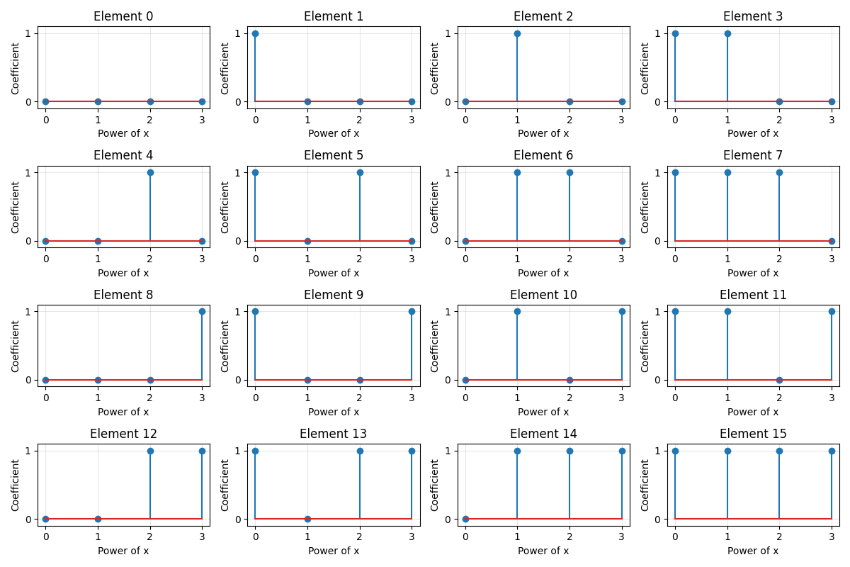
Each element of the finite field can be represented as a binary polynomial. Let’s visualize the field elements and their relationships.

# Create a visualization of field elements and their polynomial representations
elements = field.get_all_elements()

plt.figure(figsize=(12, 8))

# Create a grid to display all field elements
rows, cols = 4, 4
for i, element in enumerate(elements):
    if i < rows * cols:  # Limit to 16 elements (for GF(2^4))
        poly = element.to_polynomial()
        coeffs = poly_to_coeff_array(poly, field.m - 1)

        plt.subplot(rows, cols, i + 1)
        plt.stem(np.arange(len(coeffs)), coeffs)
        plt.title(f"Element {element}")
        plt.xlabel("Power of x")
        plt.ylabel("Coefficient")
        plt.ylim(-0.1, 1.1)
        plt.xticks(np.arange(field.m))
        plt.yticks([0, 1])
        plt.grid(True, alpha=0.3)

plt.tight_layout()
plt.show()

Minimal Polynomials

The minimal polynomial of a field element is the monic polynomial of smallest degree that has the element as a root. These are crucial for constructing error correction codes.

# Compute minimal polynomials for field elements
min_polys = []
for i in range(1, min(11, field.size)):  # Limit to first 10 non-zero elements
    element = field(i)
    min_poly = element.minimal_polynomial()
    min_polys.append((element, min_poly))
    print(f"Minimal polynomial of {element}: {min_poly}")

Minimal polynomial of 1: x + 1
Minimal polynomial of 2: x^4 + x + 1
Minimal polynomial of 3: x^4 + x + 1
Minimal polynomial of 4: x^4 + x + 1
Minimal polynomial of 5: x^4 + x + 1
Minimal polynomial of 6: x^2 + x + 1
Minimal polynomial of 7: x^2 + x + 1
Minimal polynomial of 8: x^4 + x^3 + x^2 + x + 1
Minimal polynomial of 9: x^4 + x^3 + 1
Minimal polynomial of 10: x^4 + x^3 + x^2 + x + 1

Trace Function

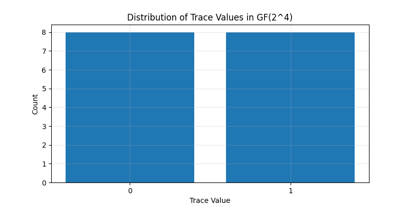
The trace function is a linear map from GF(2^m) to GF(2) that sums a field element with all its conjugates.

# Compute traces for field elements
traces = []
for i in range(field.size):
    element = field(i)
    tr = element.trace()
    traces.append(tr)
    if i < 10:  # Show only the first 10 for brevity
        print(f"Trace of {element}: {tr}")

# Plot the distribution of trace values
plt.figure(figsize=(8, 4))
labels, counts = np.unique(traces, return_counts=True)
plt.bar([str(label) for label in labels], counts)
plt.title("Distribution of Trace Values in GF(2^4)")
plt.xlabel("Trace Value")
plt.ylabel("Count")
plt.grid(True, alpha=0.3)
plt.show()

Trace of 0: 0
Trace of 1: 0
Trace of 2: 0
Trace of 3: 0
Trace of 4: 0
Trace of 5: 0
Trace of 6: 0
Trace of 7: 0
Trace of 8: 1
Trace of 9: 1

Application: Reed-Solomon Code Construction

Reed-Solomon codes are a class of non-binary cyclic error-correcting codes based on polynomial evaluation. Let’s demonstrate the basic principles behind a Reed-Solomon code using our finite field operations.

# Parameters for a simple Reed-Solomon code
m = 4  # Field GF(2^4)
n = 15  # Code length (2^m - 1)
k = 7  # Message length
t = (n - k) // 2  # Error correction capability

print(f"Constructing a Reed-Solomon({n},{k}) code over GF(2^{m})")
print(f"This code can correct up to {t} errors in a codeword of length {n}")

# Create the field
rs_field = FiniteBifield(m)
alpha = rs_field.primitive_element()

# Generate the generator polynomial g(x) = (x - α)(x - α²)...(x - α^(2t))
roots = [alpha**i for i in range(1, 2 * t + 1)]
g = BinaryPolynomial(1)  # Start with g(x) = 1

for root in roots:
    # Multiply g(x) by (x - α^i)
    # In polynomial representation, (x - α^i) = (x + α^i) since we're in characteristic 2
    factor = BinaryPolynomial(0b10)  # x
    term = BinaryPolynomial(root.value)  # α^i
    factor = BinaryPolynomial(factor.value ^ term.value)  # x + α^i
    g = g * factor

print(f"Generator polynomial: g(x) = {g}")
print(f"Degree of g(x): {g.degree} (should be 2t = {2*t})")

# Verify that the generator polynomial is not zero
if g.value == 0:
    print("Warning: Generator polynomial is zero. This is unexpected and may cause errors.")
    print("Using a default non-zero generator polynomial instead.")
    g = BinaryPolynomial(0b101)  # Using a simple polynomial x^2 + 1 as fallback

Constructing a Reed-Solomon(15,7) code over GF(2^4)
This code can correct up to 4 errors in a codeword of length 15
Generator polynomial: g(x) = 0
Degree of g(x): -1 (should be 2t = 8)
Warning: Generator polynomial is zero. This is unexpected and may cause errors.
Using a default non-zero generator polynomial instead.

Encoding Process Visualization

Let’s visualize the encoding process for a simple message.

# Create a random message polynomial of degree k-1
message_coeffs = torch.randint(0, 2, (k,))
message_poly = BinaryPolynomial(0)
for i, coeff in enumerate(message_coeffs):
    if coeff == 1:
        message_poly = BinaryPolynomial(message_poly.value ^ (1 << i))

# The encoded codeword is: c(x) = m(x)·x^(n-k) mod g(x)
shifted_message = BinaryPolynomial(message_poly.value << (n - k))

# Check if g is zero before attempting modulo operation
if g.value == 0:
    print("Error: Cannot perform modulo operation with zero polynomial.")
    remainder = BinaryPolynomial(0)
else:
    remainder = shifted_message % g

codeword_poly = BinaryPolynomial(shifted_message.value ^ remainder.value)

print(f"Message polynomial: m(x) = {message_poly}")
print(f"Encoded codeword polynomial: c(x) = {codeword_poly}")

# Visualize the encoding process
plt.figure(figsize=(12, 6))

# Plot message coefficients
plt.subplot(3, 1, 1)
message_coeffs_array = poly_to_coeff_array(message_poly, n - 1)
plt.stem(np.arange(len(message_coeffs_array)), message_coeffs_array)
plt.title("Message Polynomial Coefficients")
plt.xlabel("Power of x")
plt.ylabel("Coefficient")
plt.ylim(-0.1, 1.1)
plt.grid(True, alpha=0.3)

# Plot shifted message
plt.subplot(3, 1, 2)
shifted_coeffs_array = poly_to_coeff_array(shifted_message, n - 1)
plt.stem(np.arange(len(shifted_coeffs_array)), shifted_coeffs_array)
plt.title("Shifted Message (multiplied by x^(n-k))")
plt.xlabel("Power of x")
plt.ylabel("Coefficient")
plt.ylim(-0.1, 1.1)
plt.grid(True, alpha=0.3)

# Plot final codeword
plt.subplot(3, 1, 3)
codeword_coeffs_array = poly_to_coeff_array(codeword_poly, n - 1)
plt.stem(np.arange(len(codeword_coeffs_array)), codeword_coeffs_array)
plt.title("Final Codeword Polynomial")
plt.xlabel("Power of x")
plt.ylabel("Coefficient")
plt.ylim(-0.1, 1.1)
plt.grid(True, alpha=0.3)

plt.tight_layout()
plt.show()

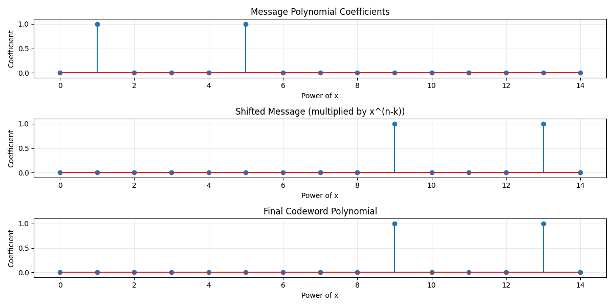
Message polynomial: m(x) = x^5 + x
Encoded codeword polynomial: c(x) = x^13 + x^9

Error Simulation and Syndrome Calculation

Let’s introduce some errors to our codeword and calculate the syndromes, which are essential for error localization in algebraic decoding.

# Convert codeword polynomial to coefficient vector
codeword = torch.tensor(codeword_poly.to_coefficient_list())
if len(codeword) < n:
    codeword = torch.cat([codeword, torch.zeros(n - len(codeword), dtype=torch.int64)])
else:
    codeword = codeword[:n]

# Introduce some errors
num_errors = t
error_positions = torch.randperm(n)[:num_errors]
received = codeword.clone()
for pos in error_positions:
    received[pos] = 1 - received[pos]  # Flip the bit

print(f"Introduced {num_errors} errors at positions: {error_positions.tolist()}")

# Calculate syndromes - evaluate the received polynomial at α, α², ..., α^(2t)
syndromes = []
received_poly = BinaryPolynomial(0)
for i, coeff in enumerate(received):
    if coeff == 1:
        received_poly = BinaryPolynomial(received_poly.value ^ (1 << i))

for i in range(1, 2 * t + 1):
    point = alpha**i
    evaluation = received_poly.evaluate(point)
    syndromes.append(evaluation.value)
    print(f"S_{i} = r(α^{i}) = {evaluation}")

# Visualize errors and syndromes
plt.figure(figsize=(12, 8))

# Plot original codeword
plt.subplot(3, 1, 1)
plt.stem(np.arange(n), codeword.numpy())
plt.title("Original Codeword")
plt.xlabel("Position")
plt.ylabel("Bit Value")
plt.ylim(-0.1, 1.1)
plt.grid(True, alpha=0.3)

# Plot received vector with errors
plt.subplot(3, 1, 2)
plt.stem(np.arange(n), received.numpy())
plt.title("Received Vector with Errors")
plt.xlabel("Position")
plt.ylabel("Bit Value")
plt.ylim(-0.1, 1.1)
# Highlight error positions
for pos in error_positions:
    plt.scatter(pos, received[pos], color="red", s=100, marker="x", zorder=5)
plt.grid(True, alpha=0.3)

# Plot syndrome values
plt.subplot(3, 1, 3)
syndrome_values = np.array(syndromes)
plt.stem(np.arange(1, len(syndromes) + 1), syndrome_values)
plt.title("Syndrome Values")
plt.xlabel("Syndrome Index")
plt.ylabel("Value in GF(2^4)")
plt.grid(True, alpha=0.3)

plt.tight_layout()
plt.show()

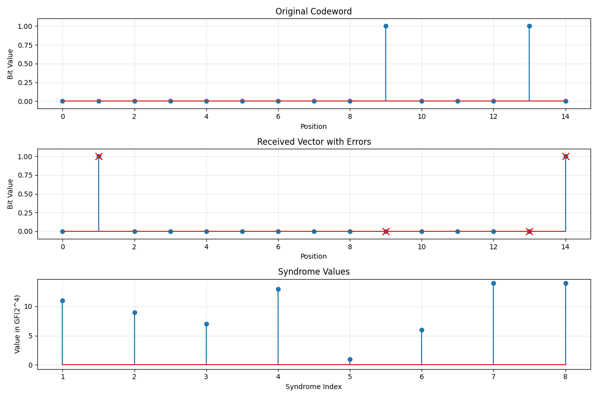
Introduced 4 errors at positions: [14, 1, 9, 13]
S_1 = r(α^1) = 11
S_2 = r(α^2) = 9
S_3 = r(α^3) = 7
S_4 = r(α^4) = 13
S_5 = r(α^5) = 1
S_6 = r(α^6) = 6
S_7 = r(α^7) = 14
S_8 = r(α^8) = 14

Conclusion

In this example, we’ve explored the algebraic foundations of forward error correction codes using the binary polynomial and finite field utilities in Kaira:

Key points: - Binary polynomials provide the mathematical basis for operations in GF(2) - Finite fields (Galois fields) extend these operations to larger fields - Reed-Solomon codes leverage finite field properties for powerful error correction - The encoding process involves polynomial operations in the finite field - Syndromes are calculated by evaluating the received polynomial at powers of a primitive field element

These algebraic structures form the foundation for many advanced error correction codes used in storage systems, communication technologies, and digital transmission.

References: - [Lin and Costello, 2004] - Provides fundamentals and applications of error control coding - [Moon, 2005] - Mathematical methods and algorithms for error correction - [Berlekamp, 1968] - Classic text on algebraic coding theory - [Blahut, 2003] - Comprehensive reference on algebraic codes for data transmission - [Reed, 1954] - Original paper on Reed-Solomon codes - [Massey, 1969] - Key paper on efficient BCH decoding