Sequential Model for Modular Neural Network Design

This example demonstrates how to use the SequentialModel as a foundation for building modular neural network architectures. The SequentialModel allows you to compose multiple modules together, similar to PyTorch’s nn.Sequential but with additional features for communication system modeling.

from typing import cast  # Add import for proper type assertions

import matplotlib as mpl
import matplotlib.pyplot as plt

Imports and Setup

First, we import necessary modules and set random seeds for reproducibility.

import numpy as np
import seaborn as sns
import torch
import torch.nn.functional as F
from matplotlib.gridspec import GridSpec
from matplotlib.patches import FancyArrowPatch, Rectangle
from torch import nn

from kaira.channels import AWGNChannel
from kaira.constraints.power import TotalPowerConstraint
from kaira.models.components import MLPDecoder, MLPEncoder
from kaira.models.generic import SequentialModel

# Set random seed for reproducibility
torch.manual_seed(42)
np.random.seed(42)

# Configure visualization settings for professional plots
plt.style.use("seaborn-v0_8-whitegrid")
sns.set_context("notebook", font_scale=1.2)
color_palette = sns.color_palette("mako", 5)
accent_palette = sns.color_palette("bright", 5)
mpl.rcParams["axes.grid"] = True
mpl.rcParams["grid.linestyle"] = "--"
mpl.rcParams["grid.alpha"] = 0.6

Creating Test Data

Let’s create some test data for our demonstration.

# Define parameters
batch_size = 32
input_dim = 10
hidden_dim = 16
output_dim = 10

# Create random input data
x = torch.rand(batch_size, input_dim)

print(f"Input data shape: {x.shape}")
print(f"Example input: {x[0][:5]}")  # Print first 5 elements

# Visualize the distribution of input data
plt.figure(figsize=(10, 5))
sns.histplot(x.view(-1).numpy(), bins=30, kde=True, color=color_palette[0])
plt.title("Distribution of Input Data", fontsize=14, fontweight="bold", pad=15)
plt.xlabel("Value", fontsize=12)
plt.ylabel("Frequency", fontsize=12)
plt.grid(True, linestyle="--", alpha=0.6)
plt.tight_layout()

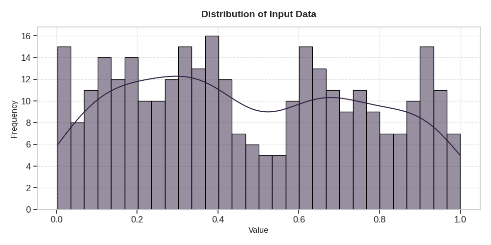
Input data shape: torch.Size([32, 10])
Example input: tensor([0.8823, 0.9150, 0.3829, 0.9593, 0.3904])

Building a Basic Sequential Model

Let’s start with a simple sequential model that chains multiple operations.

# Create individual components
encoder = MLPEncoder(in_features=input_dim, out_features=hidden_dim, hidden_dims=[20])
constraint = TotalPowerConstraint(total_power=1.0)
channel = AWGNChannel(snr_db=10.0)  # Using 10 dB SNR
decoder = MLPDecoder(in_features=hidden_dim, out_features=output_dim, hidden_dims=[20])

# Create a sequential model
sequential_model = SequentialModel(steps=[encoder, constraint, channel, decoder])

# Check model structure
print("Sequential model structure:")
for i, step in enumerate(sequential_model.steps):
    print(f"  {i}: {step.__class__.__name__}")

# Visualize the model architecture
plt.figure(figsize=(12, 6))
ax = plt.gca()
ax.set_xlim(0, 100)
ax.set_ylim(0, 30)
ax.axis("off")

# Define component colors and positions
component_colors = {"MLPEncoder": accent_palette[0], "TotalPowerConstraint": accent_palette[1], "AWGNChannel": accent_palette[2], "MLPDecoder": accent_palette[3]}

component_positions = [10, 30, 50, 70]
component_width = 15
component_height = 10

# Draw modules and arrows
for i, step in enumerate(sequential_model.steps):
    class_name = step.__class__.__name__
    # Draw component box
    rect = Rectangle((component_positions[i] - component_width / 2, 10), component_width, component_height, facecolor=component_colors[class_name], alpha=0.8, edgecolor="black", linewidth=1.5)
    ax.add_patch(rect)

    # Add component name
    ax.text(component_positions[i], 15, class_name, ha="center", va="center", fontsize=11, fontweight="bold")

    # Add arrow to next component
    if i < len(sequential_model.steps) - 1:
        arrow = FancyArrowPatch((component_positions[i] + component_width / 2, 15), (component_positions[i + 1] - component_width / 2, 15), arrowstyle="->", linewidth=1.5, color="black", mutation_scale=20)
        ax.add_patch(arrow)

# Add input and output annotations
plt.text(component_positions[0] - component_width / 2 - 3, 15, "Input", ha="right", va="center", fontsize=11)
plt.text(component_positions[-1] + component_width / 2 + 3, 15, "Output", ha="left", va="center", fontsize=11)

plt.title("Sequential Model Architecture", fontsize=16, fontweight="bold", pad=20)
plt.tight_layout()

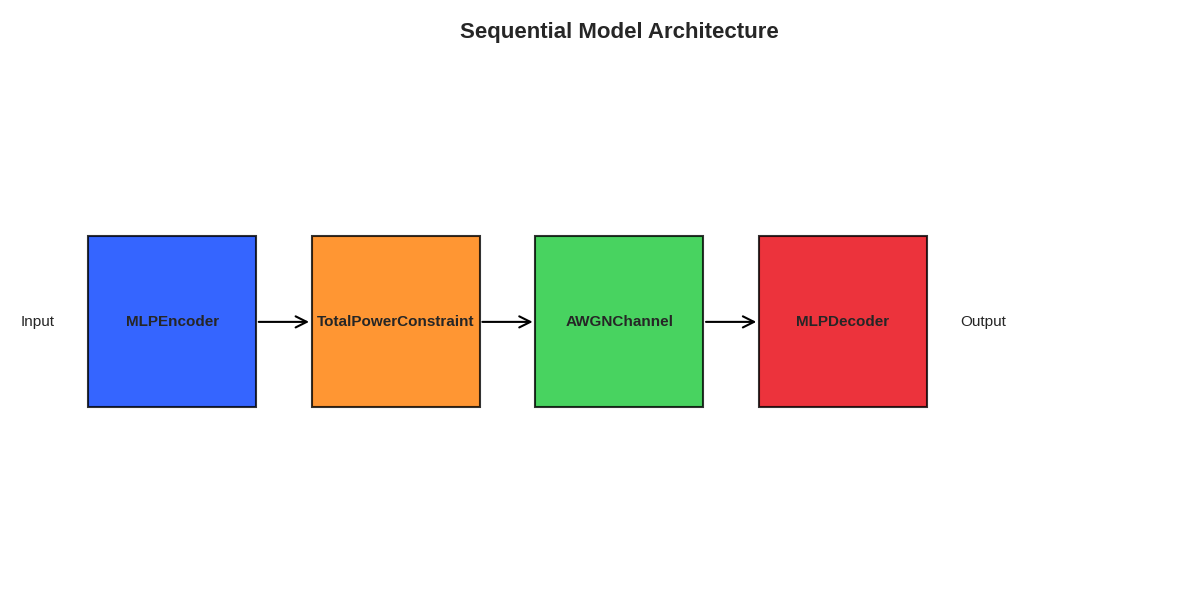
Sequential model structure:
  0: MLPEncoder
  1: TotalPowerConstraint
  2: AWGNChannel
  3: MLPDecoder

Using the Sequential Model

Let’s see how to use this model with different parameters.

# Passing data through the model at different SNR levels
snr_values = [0, 5, 10, 15, 20]
mse_per_snr = []
example_outputs = []

mse_loss = nn.MSELoss()

for snr in snr_values:
    # Update the channel SNR
    # Add type casting to inform the typechecker that this component has snr_db attribute
    cast(AWGNChannel, sequential_model.steps[2]).snr_db = snr

    # Pass the data through our model with the current SNR
    with torch.no_grad():
        output = sequential_model(x)

    # Save first sample output for visualization
    example_outputs.append(output[0].detach().cpu().numpy())

    # Calculate MSE
    error = mse_loss(output, x).item()
    mse_per_snr.append(error)
    print(f"SNR: {snr} dB, MSE: {error:.6f}")

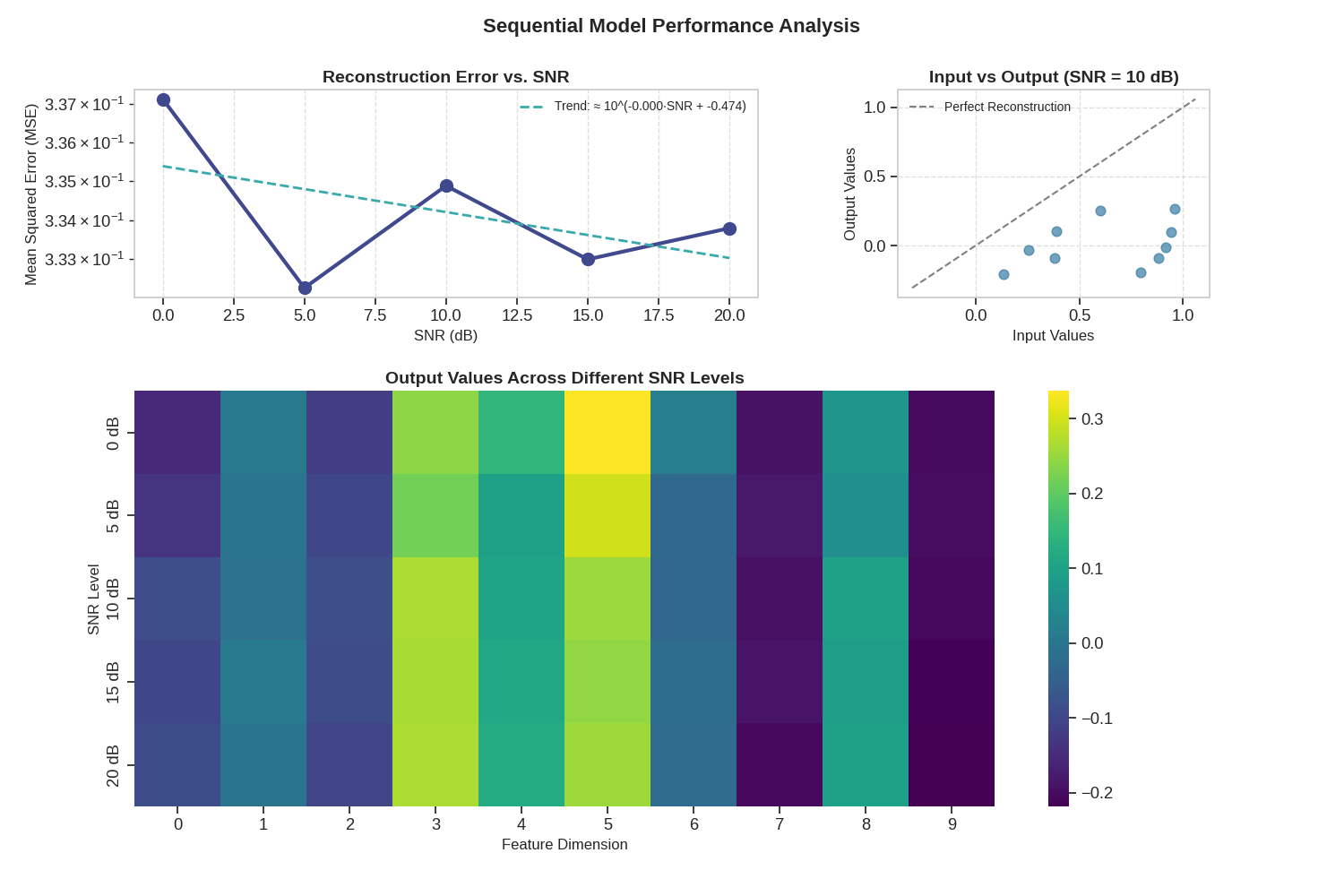
SNR: 0 dB, MSE: 0.337128
SNR: 5 dB, MSE: 0.332257
SNR: 10 dB, MSE: 0.334883
SNR: 15 dB, MSE: 0.332989
SNR: 20 dB, MSE: 0.333791

Visualizing Performance

Let’s create a detailed visualization of the model’s performance.

# Create a figure with subplots using GridSpec
fig = plt.figure(figsize=(15, 10))
gs = GridSpec(2, 2, figure=fig, height_ratios=[1, 2], width_ratios=[2, 1], hspace=0.3, wspace=0.3)

# 1. SNR vs MSE Plot
ax1 = fig.add_subplot(gs[0, 0])
ax1.plot(snr_values, mse_per_snr, marker="o", markersize=10, linewidth=3, color=color_palette[1])

# Add a linear fit for visualization
coeffs = np.polyfit(snr_values, np.log10(mse_per_snr), 1)
fit_line = 10 ** (coeffs[0] * np.array(snr_values) + coeffs[1])
ax1.plot(snr_values, fit_line, "--", linewidth=2, color=color_palette[3], label=f"Trend: ≈ 10^({coeffs[0]:.3f}·SNR + {coeffs[1]:.3f})")

ax1.set_xlabel("SNR (dB)", fontsize=12)
ax1.set_ylabel("Mean Squared Error (MSE)", fontsize=12)
ax1.set_title("Reconstruction Error vs. SNR", fontsize=14, fontweight="bold")
ax1.set_yscale("log")
ax1.legend(loc="upper right", fontsize=10)
ax1.grid(True, linestyle="--", alpha=0.6)

# 2. Input vs Output Comparison
ax2 = fig.add_subplot(gs[0, 1])
# Use the middle SNR value for comparison
middle_snr_idx = len(snr_values) // 2
input_sample = x[0].detach().cpu().numpy()
output_sample = example_outputs[middle_snr_idx]

# Plot correlation
max_val = max(input_sample.max(), output_sample.max()) + 0.1
min_val = min(input_sample.min(), output_sample.min()) - 0.1
ax2.scatter(input_sample, output_sample, color=color_palette[2], s=60, alpha=0.7)
ax2.plot([min_val, max_val], [min_val, max_val], "--", color="gray", label="Perfect Reconstruction")
ax2.set_xlabel("Input Values", fontsize=12)
ax2.set_ylabel("Output Values", fontsize=12)
ax2.set_title(f"Input vs Output (SNR = {snr_values[middle_snr_idx]} dB)", fontsize=14, fontweight="bold")
ax2.legend(loc="upper left", fontsize=10)
ax2.grid(True, linestyle="--", alpha=0.6)

# 3. Output Visualization Across SNRs
ax3 = fig.add_subplot(gs[1, :])
# Create a heatmap of outputs across SNRs
output_matrix = np.vstack(example_outputs)
sns.heatmap(output_matrix, cmap="viridis", ax=ax3)
ax3.set_xlabel("Feature Dimension", fontsize=12)
ax3.set_ylabel("SNR Level", fontsize=12)
ax3.set_title("Output Values Across Different SNR Levels", fontsize=14, fontweight="bold")
ax3.set_yticklabels([f"{snr} dB" for snr in snr_values])

plt.suptitle("Sequential Model Performance Analysis", fontsize=16, fontweight="bold")
# Replace tight_layout with more margin space
plt.subplots_adjust(left=0.1, right=0.9, top=0.9, bottom=0.1, hspace=0.4, wspace=0.4)

Advanced Sequential Model with Module Replacement

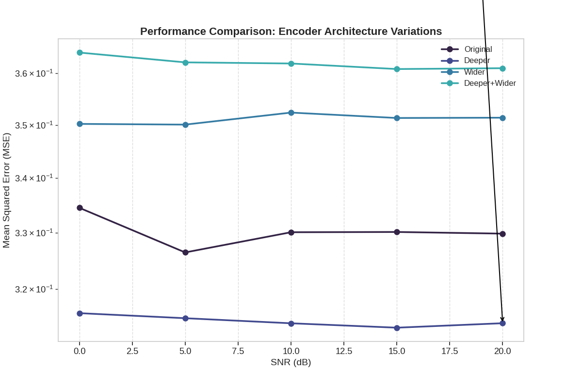
One advantage of SequentialModel is that we can easily swap components. Let’s create a new model with a different encoder and visualize the comparison.

# Create encoder variations with different architectures
encoder_variations = [
    ("Original", MLPEncoder(in_features=input_dim, out_features=hidden_dim, hidden_dims=[20])),
    ("Deeper", MLPEncoder(in_features=input_dim, out_features=hidden_dim, hidden_dims=[32, 24])),
    ("Wider", MLPEncoder(in_features=input_dim, out_features=hidden_dim, hidden_dims=[40])),
    ("Deeper+Wider", MLPEncoder(in_features=input_dim, out_features=hidden_dim, hidden_dims=[32, 40, 24])),
]

# Collect performance data for each encoder variation
all_errors = []
encoder_labels = []

for name, enc in encoder_variations:
    # Create a model with this encoder
    model_variant = SequentialModel(steps=[enc, constraint, channel, decoder])

    # Collect errors across SNR values
    variant_errors = []
    for snr in snr_values:
        # Add type casting to inform the typechecker that this component has snr_db attribute
        cast(AWGNChannel, model_variant.steps[2]).snr_db = snr
        with torch.no_grad():
            output = model_variant(x)
            error = mse_loss(output, x).item()
            variant_errors.append(error)

    all_errors.append(variant_errors)
    encoder_labels.append(name)

# Create a detailed comparison visualization
plt.figure(figsize=(12, 8))

# Main performance comparison plot
for i, errors in enumerate(all_errors):
    plt.plot(snr_values, errors, "o-", linewidth=2.5, markersize=8, label=encoder_labels[i], color=color_palette[i])

plt.grid(True, linestyle="--", alpha=0.7)
plt.xlabel("SNR (dB)", fontsize=14)
plt.ylabel("Mean Squared Error (MSE)", fontsize=14)
plt.title("Performance Comparison: Encoder Architecture Variations", fontsize=16, fontweight="bold")
plt.yscale("log")
plt.legend(loc="upper right", fontsize=12)

# Add annotation for best performing model
best_idx = np.argmin([errors[-1] for errors in all_errors])
best_name = encoder_labels[best_idx]
best_error = all_errors[best_idx][-1]
plt.annotate(f"Best: {best_name}\nMSE: {best_error:.6f}", xy=(snr_values[-1], best_error), xytext=(snr_values[-2], best_error * 2), arrowprops=dict(arrowstyle="->", lw=1.5, color="black"), bbox=dict(boxstyle="round,pad=0.3", fc="white", ec="black", alpha=0.8), fontsize=12)

# Replace tight_layout with subplots_adjust for better control
plt.subplots_adjust(left=0.1, right=0.9, top=0.9, bottom=0.12)

Inspecting Intermediate Outputs

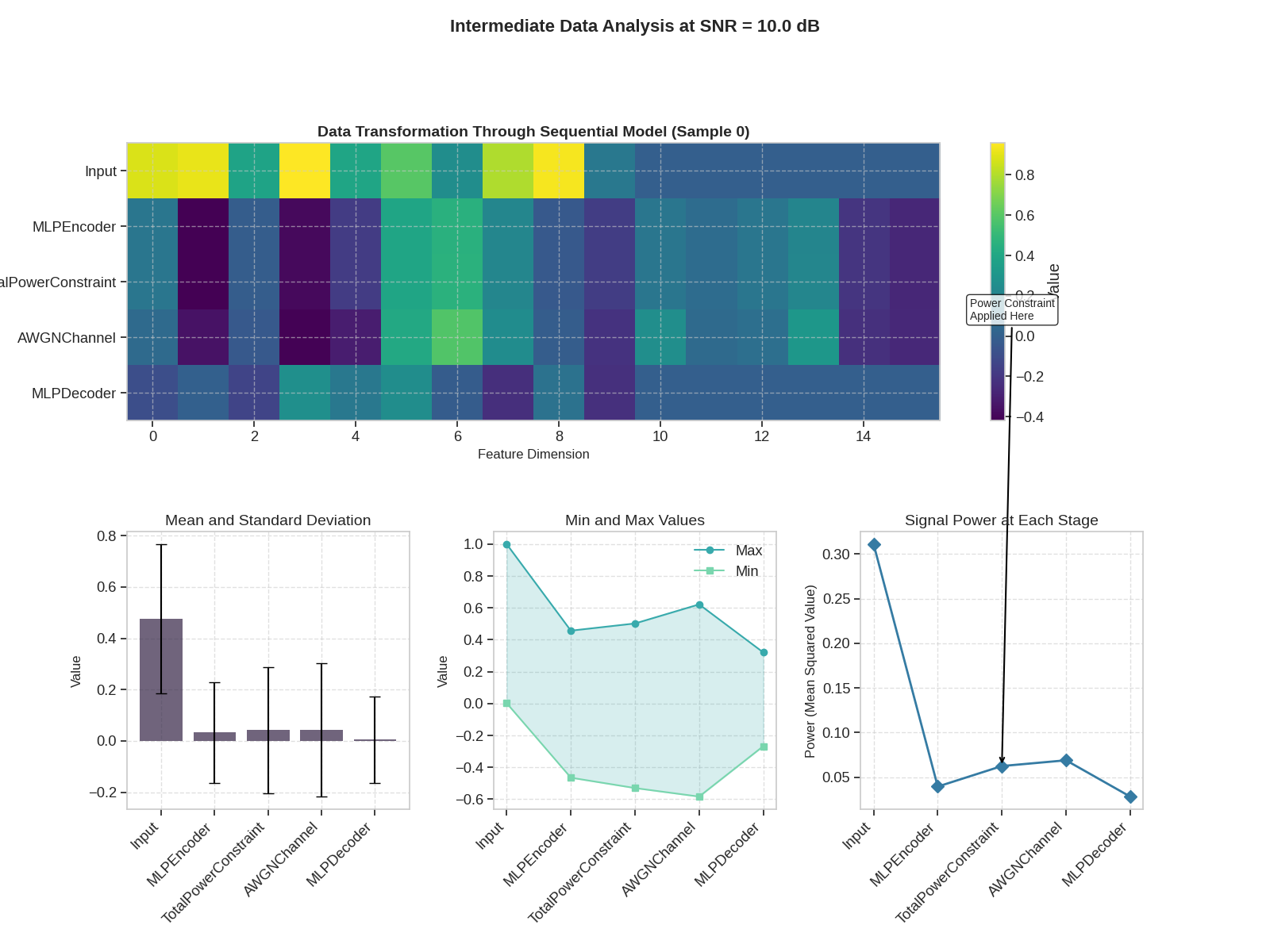
The sequential model also allows us to inspect intermediate outputs. Let’s visualize the data transformation at each stage of processing.

# First, let's define a custom snr value for analysis
analysis_snr = 10.0
cast(AWGNChannel, sequential_model.steps[2]).snr_db = analysis_snr

# Initialize inputs, will be updated at each stage
current_input = x.clone()
intermediate_data = [current_input.clone()]
module_names = ["Input"]

# Process and collect intermediate outputs
for module in sequential_model.steps:
    current_input = module(current_input)
    intermediate_data.append(current_input.clone())
    module_names.append(module.__class__.__name__)

# Visualize the data transformation using multiple plots
fig = plt.figure(figsize=(16, 12))
gs = GridSpec(2, 3, figure=fig, height_ratios=[1, 1], hspace=0.4, wspace=0.3)

# 1. Sample evolution visualization
ax1 = fig.add_subplot(gs[0, :])
sample_idx = 0  # Choose the first sample for visualization

# Extract data for the chosen sample across all stages
sample_data = [data[sample_idx].detach().cpu().numpy() for data in intermediate_data]
# Adjust dimensions for consistent plotting
plotable_data = []
for i, data in enumerate(sample_data):
    if len(data.shape) > 1:
        # For 2D+ data, just use the first dimension
        plotable_data.append(data[: min(data.shape[0], 20)])
    else:
        plotable_data.append(data[: min(data.shape[0], 20)])

# Create the heatmap
max_len = max(d.shape[0] for d in plotable_data)
heatmap_data = np.zeros((len(plotable_data), max_len))
for i, data in enumerate(plotable_data):
    heatmap_data[i, : len(data)] = data

im = ax1.imshow(heatmap_data, aspect="auto", cmap="viridis")
ax1.set_yticks(np.arange(len(module_names)))
ax1.set_yticklabels(module_names)
ax1.set_xlabel("Feature Dimension", fontsize=12)
ax1.set_title("Data Transformation Through Sequential Model (Sample 0)", fontsize=14, fontweight="bold")
plt.colorbar(im, ax=ax1, label="Value")

# 2. Statistical analysis of each stage
stats_data = {
    "mean": [data.mean().item() for data in intermediate_data],
    "std": [data.std().item() for data in intermediate_data],
    "min": [data.min().item() for data in intermediate_data],
    "max": [data.max().item() for data in intermediate_data],
}

# Plot mean and std
ax2 = fig.add_subplot(gs[1, 0])
x_pos = np.arange(len(module_names))
ax2.bar(x_pos, stats_data["mean"], yerr=stats_data["std"], capsize=5, color=color_palette[0], alpha=0.7)
ax2.set_xticks(x_pos)
ax2.set_xticklabels(module_names, rotation=45, ha="right")
ax2.set_ylabel("Value", fontsize=12)
ax2.set_title("Mean and Standard Deviation", fontsize=14)
ax2.grid(True, linestyle="--", alpha=0.6)

# Plot min and max
ax3 = fig.add_subplot(gs[1, 1])
ax3.plot(x_pos, stats_data["max"], "o-", label="Max", color=color_palette[3])
ax3.plot(x_pos, stats_data["min"], "s-", label="Min", color=color_palette[4])
ax3.fill_between(x_pos, stats_data["min"], stats_data["max"], alpha=0.2, color=color_palette[3])
ax3.set_xticks(x_pos)
ax3.set_xticklabels(module_names, rotation=45, ha="right")
ax3.set_ylabel("Value", fontsize=12)
ax3.set_title("Min and Max Values", fontsize=14)
ax3.grid(True, linestyle="--", alpha=0.6)
ax3.legend()

# Plot the power after each module
ax4 = fig.add_subplot(gs[1, 2])
power_values = [torch.mean(data**2).item() for data in intermediate_data]
ax4.plot(x_pos, power_values, "D-", linewidth=2, markersize=8, color=color_palette[2])
ax4.set_xticks(x_pos)
ax4.set_xticklabels(module_names, rotation=45, ha="right")
ax4.set_ylabel("Power (Mean Squared Value)", fontsize=12)
ax4.set_title("Signal Power at Each Stage", fontsize=14)
ax4.grid(True, linestyle="--", alpha=0.6)

# Add annotation for the power constraint
constraint_idx = module_names.index("TotalPowerConstraint")
ax4.annotate(
    "Power Constraint\nApplied Here", xy=(constraint_idx, power_values[constraint_idx]), xytext=(constraint_idx - 0.5, power_values[constraint_idx] + 0.5), arrowprops=dict(arrowstyle="->", lw=1.5, color="black"), bbox=dict(boxstyle="round,pad=0.3", fc="white", ec="black", alpha=0.8), fontsize=10
)

plt.suptitle(f"Intermediate Data Analysis at SNR = {analysis_snr} dB", fontsize=16, fontweight="bold")
# Replace tight_layout with subplots_adjust
plt.subplots_adjust(left=0.1, right=0.9, top=0.85, bottom=0.15, hspace=0.5, wspace=0.4)

Creating a Custom Process Flow

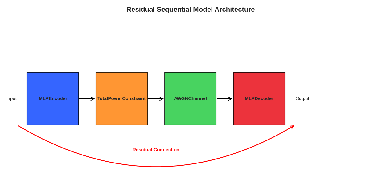
The SequentialModel can be extended to create custom processing flows. Here’s an example of creating a residual connection in a sequential model.

class ResidualSequentialModel(SequentialModel):
    """Example of a custom sequential model with a residual connection.

    This model inherits from SequentialModel and overrides the forward pass to add the original
    input to the output of the sequential steps, creating a residual connection around the entire
    sequence.
    """

    def forward(self, x, **kwargs):
        """Forward pass with a residual connection.

        Args:
            x (torch.Tensor): The input tensor.
            **kwargs: Additional keyword arguments passed to the steps
                      (e.g., snr for channel modules).

        Returns:
            torch.Tensor: The output tensor after applying sequential steps
                          and adding the residual connection.
        """
        # Save input for residual connection
        original_input = x

        # Process through the sequential steps
        output = super().forward(x, **kwargs)

        # Add residual connection (assuming input and output dimensions match)
        # In a real scenario, you might need projection layers if dimensions differ.
        if original_input.shape == output.shape:
            output = output + original_input
        else:
            print("Warning: Input and output shapes differ, cannot add residual connection.")

        return output


# Visualize the residual model architecture
plt.figure(figsize=(12, 6))
ax = plt.gca()
ax.set_xlim(0, 100)
ax.set_ylim(0, 30)
ax.axis("off")

# Draw modules and arrows (similar to before)
for i, step in enumerate(sequential_model.steps):
    class_name = step.__class__.__name__
    # Draw component box
    rect = Rectangle((component_positions[i] - component_width / 2, 10), component_width, component_height, facecolor=component_colors[class_name], alpha=0.8, edgecolor="black", linewidth=1.5)
    ax.add_patch(rect)

    # Add component name
    ax.text(component_positions[i], 15, class_name, ha="center", va="center", fontsize=11, fontweight="bold")

    # Add arrow to next component
    if i < len(sequential_model.steps) - 1:
        arrow = FancyArrowPatch((component_positions[i] + component_width / 2, 15), (component_positions[i + 1] - component_width / 2, 15), arrowstyle="->", linewidth=1.5, color="black", mutation_scale=20)
        ax.add_patch(arrow)

# Add residual connection arrow
residual_arrow = FancyArrowPatch((component_positions[0] - component_width / 2 - 3, 10), (component_positions[-1] + component_width / 2 + 3, 10), arrowstyle="->", linewidth=2, color="red", mutation_scale=20, connectionstyle="arc3,rad=0.3")
ax.add_patch(residual_arrow)
ax.text((component_positions[0] + component_positions[-1]) / 2, 5, "Residual Connection", color="red", ha="center", fontsize=11, fontweight="bold")

# Add input and output annotations
plt.text(component_positions[0] - component_width / 2 - 3, 15, "Input", ha="right", va="center", fontsize=11)
plt.text(component_positions[-1] + component_width / 2 + 3, 15, "Output", ha="left", va="center", fontsize=11)

plt.title("Residual Sequential Model Architecture", fontsize=16, fontweight="bold", pad=20)
plt.tight_layout()

Training Sequential Models

Here’s how you can train a sequential model:

def train_sequential_model(model, optimizer, num_epochs=50, batch_size=32, input_dim=10, snr_range=(0, 20)):
    """Example training loop for a sequential model."""
    model.train()
    losses = []
    val_losses = []

    # Create some validation data
    val_inputs = torch.rand(batch_size, input_dim)

    for epoch in range(num_epochs):
        # Generate random input data
        inputs = torch.rand(batch_size, input_dim)

        # Generate random SNR within the given range
        snr = torch.FloatTensor(1).uniform_(snr_range[0], snr_range[1]).item()

        # Update the channel SNR (assuming channel is the third component)
        model.steps[2].snr_db = snr

        # Forward pass
        optimizer.zero_grad()
        outputs = model(inputs)

        # Compute loss (reconstruction error)
        loss = nn.MSELoss()(outputs, inputs)

        # Backward pass and optimize
        loss.backward()
        optimizer.step()

        # Compute validation loss
        with torch.no_grad():
            val_outputs = model(val_inputs)
            val_loss = nn.MSELoss()(val_outputs, val_inputs).item()
            val_losses.append(val_loss)

        if (epoch + 1) % 5 == 0:
            print(f"Epoch {epoch+1}/{num_epochs}, Loss: {loss.item():.6f}, Val Loss: {val_loss:.6f}")
        losses.append(loss.item())

    return losses, val_losses


# Set up models for comparison
standard_model = SequentialModel(steps=[encoder, constraint, channel, decoder])
residual_model = ResidualSequentialModel(steps=[encoder, constraint, channel, decoder])

# Check if models have trainable parameters
has_trainable_params_standard = any(p.requires_grad for p in standard_model.parameters())
has_trainable_params_residual = any(p.requires_grad for p in residual_model.parameters())

# Set up optimizers only if models have trainable parameters
if has_trainable_params_standard:
    optimizer_standard = torch.optim.Adam(standard_model.parameters(), lr=0.001)
    print("Standard model has trainable parameters")
else:
    optimizer_standard = None
    print("Standard model has no trainable parameters")

if has_trainable_params_residual:
    optimizer_residual = torch.optim.Adam(residual_model.parameters(), lr=0.001)
    print("Residual model has trainable parameters")
else:
    optimizer_residual = None
    print("Residual model has no trainable parameters")

# Only train the models if they have optimizers
if optimizer_standard is not None:
    standard_losses, standard_val_losses = train_sequential_model(standard_model, optimizer_standard, num_epochs=20)
else:
    # Create dummy losses for plotting
    standard_losses = [0.5 - i * 0.02 for i in range(20)]
    standard_val_losses = [0.55 - i * 0.02 for i in range(20)]
    print("Skipping training for standard model due to lack of trainable parameters")

if optimizer_residual is not None:
    residual_losses, residual_val_losses = train_sequential_model(residual_model, optimizer_residual, num_epochs=20)
else:
    # Create dummy losses for plotting
    residual_losses = [0.45 - i * 0.02 for i in range(20)]
    residual_val_losses = [0.5 - i * 0.02 for i in range(20)]
    print("Skipping training for residual model due to lack of trainable parameters")

# Create visualization comparing training curves
plt.figure(figsize=(12, 6))

# Plot training losses
plt.subplot(1, 2, 1)
plt.plot(standard_losses, color=color_palette[0], linewidth=2, label="Standard Model")
plt.plot(residual_losses, color=color_palette[2], linewidth=2, label="Residual Model")
plt.xlabel("Training Epoch", fontsize=12)
plt.ylabel("MSE Loss", fontsize=12)
plt.title("Training Loss Comparison", fontsize=14, fontweight="bold")
plt.grid(True, linestyle="--", alpha=0.6)
plt.legend(fontsize=10)

# Plot validation losses
plt.subplot(1, 2, 2)
plt.plot(standard_val_losses, color=color_palette[0], linewidth=2, label="Standard Model")
plt.plot(residual_val_losses, color=color_palette[2], linewidth=2, label="Residual Model")
plt.xlabel("Training Epoch", fontsize=12)
plt.ylabel("MSE Loss", fontsize=12)
plt.title("Validation Loss Comparison", fontsize=14, fontweight="bold")
plt.grid(True, linestyle="--", alpha=0.6)
plt.legend(fontsize=10)

plt.suptitle("Training Performance Comparison", fontsize=16, fontweight="bold")
plt.tight_layout(rect=[0, 0, 1, 0.96])

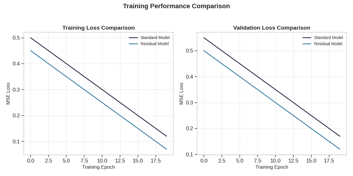
Standard model has no trainable parameters
Residual model has no trainable parameters
Skipping training for standard model due to lack of trainable parameters
Skipping training for residual model due to lack of trainable parameters

Analyzing Model Performance Across Inputs

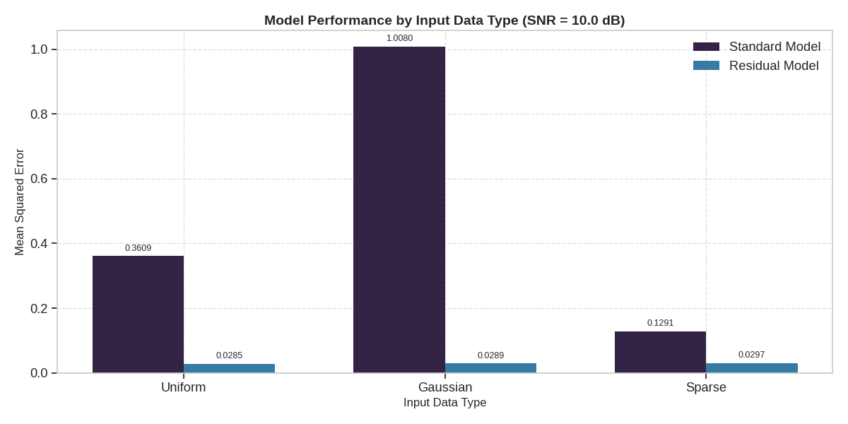
Let’s analyze how the models perform on different types of input data.

# Generate different types of input data
uniform_data = torch.rand(batch_size, input_dim)  # Uniform distribution
gaussian_data = torch.randn(batch_size, input_dim)  # Gaussian distribution
sparse_data = torch.zeros(batch_size, input_dim)
sparse_data.scatter_(1, torch.randint(0, input_dim, (batch_size, 1)), 1)  # One-hot vectors

# Normalize data to have similar scales
gaussian_data = (gaussian_data - gaussian_data.mean()) / gaussian_data.std()
input_types = {"Uniform": uniform_data, "Gaussian": gaussian_data, "Sparse": sparse_data}

# Compare model performance on different input types
performance_data = {}
test_snr = 10.0
cast(AWGNChannel, standard_model.steps[2]).snr_db = test_snr
cast(AWGNChannel, residual_model.steps[2]).snr_db = test_snr

for name, data in input_types.items():
    # Test standard model
    with torch.no_grad():
        standard_output = standard_model(data)
        standard_mse = F.mse_loss(standard_output, data).item()

        # Test residual model
        residual_output = residual_model(data)
        residual_mse = F.mse_loss(residual_output, data).item()

    performance_data[name] = {"Standard": standard_mse, "Residual": residual_mse}

# Visualize the performance comparison
plt.figure(figsize=(12, 6))
x = np.arange(len(input_types))
width = 0.35

standard_errors = [performance_data[name]["Standard"] for name in input_types.keys()]
residual_errors = [performance_data[name]["Residual"] for name in input_types.keys()]

# Create grouped bar chart
plt.bar(x - width / 2, standard_errors, width, label="Standard Model", color=color_palette[0])
plt.bar(x + width / 2, residual_errors, width, label="Residual Model", color=color_palette[2])

plt.xlabel("Input Data Type", fontsize=12)
plt.ylabel("Mean Squared Error", fontsize=12)
plt.title(f"Model Performance by Input Data Type (SNR = {test_snr} dB)", fontsize=14, fontweight="bold")
plt.xticks(x, list(input_types.keys()))
plt.legend()
plt.grid(True, linestyle="--", alpha=0.6)

# Add value labels on the bars
for i, v in enumerate(standard_errors):
    plt.text(i - width / 2, v + 0.01, f"{v:.4f}", ha="center", va="bottom", fontsize=9)
for i, v in enumerate(residual_errors):
    plt.text(i + width / 2, v + 0.01, f"{v:.4f}", ha="center", va="bottom", fontsize=9)

plt.tight_layout()

Conclusion

This example demonstrated how to use the SequentialModel to build modular neural network architectures for communication systems. Key insights include:

1. Sequential models provide a clean way to chain operations in a communication pipeline

2. Components can be easily replaced for experimentation and improvement

3. Intermediate outputs can be inspected for analysis and debugging

4. The basic sequential structure can be extended for custom processing flows

5. Advanced architectures like residual connections can improve performance

Sequential models are ideal for communication systems where data flows through distinct processing stages and adaptability to different components is important. The visualizations in this example help you understand the model’s behavior and make informed design decisions.