Basic Binary Operations for FEC

This example demonstrates the fundamental binary operations used in forward error correction (FEC) coding. We’ll explore how to calculate Hamming distances, Hamming weights, and convert between binary and integer representations using utility functions from the FEC module.

import matplotlib.patheffects as PathEffects
import matplotlib.pyplot as plt
import numpy as np
import seaborn as sns
import torch
from matplotlib.gridspec import GridSpec
from matplotlib.patches import CirclePolygon, FancyArrowPatch, Rectangle

from kaira.models.fec.utils import (
    from_binary_tensor,
    hamming_distance,
    hamming_weight,
    to_binary_tensor,
)

Setting up

First, we set a random seed to ensure reproducibility of results and configure our visualization settings.

torch.manual_seed(42)
np.random.seed(42)

# Configure better visualization settings
plt.style.use("seaborn-v0_8-whitegrid")
sns.set_context("notebook", font_scale=1.2)

# Create custom colormaps for our visualizations
bit_0_color = "#3498db"  # Blue
bit_1_color = "#e74c3c"  # Red
highlight_color = "#f39c12"  # Orange
difference_color = "#9b59b6"  # Purple
background_color = "#f8f9fa"  # Light gray background

# Define a modern color palette
modern_palette = sns.color_palette("viridis", 8)
accent_palette = sns.color_palette("Set2", 8)

Hamming Distance

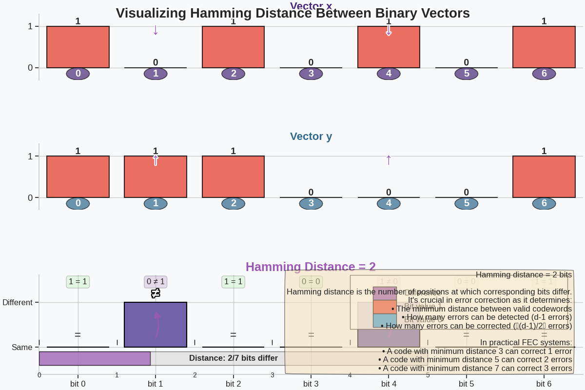
The Hamming distance is a fundamental metric in coding theory, representing the number of positions at which corresponding symbols differ between two strings. In FEC, it directly relates to the error detection and correction capabilities.

Let’s compute the Hamming distance between some binary vectors:

# Create binary vectors
x = torch.tensor([1, 0, 1, 0, 1, 0, 1])
y = torch.tensor([1, 1, 1, 0, 0, 0, 1])

# Calculate Hamming distance
dist = hamming_distance(x, y)

print(f"Vector x: {x}")
print(f"Vector y: {y}")
print(f"Hamming distance: {dist}")

Vector x: tensor([1, 0, 1, 0, 1, 0, 1])
Vector y: tensor([1, 1, 1, 0, 0, 0, 1])
Hamming distance: 2

Visualizing Hamming Distance

We can visualize the binary vectors and highlight the positions where they differ using an interactive and informative visualization.

fig = plt.figure(figsize=(12, 8), facecolor=background_color, constrained_layout=True)
gs = GridSpec(3, 1, figure=fig, height_ratios=[1, 1, 1.5], hspace=0.4)

# Plot the first vector
ax1 = fig.add_subplot(gs[0], facecolor=background_color)
ax1.set_title("Vector x", fontsize=16, fontweight="bold", color=modern_palette[0])
bars1 = ax1.bar(np.arange(len(x)), x.numpy(), color=[bit_1_color if bit == 1 else bit_0_color for bit in x], edgecolor="black", linewidth=1.5, alpha=0.8)

# Add value labels with better styling
for i, v in enumerate(x):
    txt = ax1.text(i, v + 0.05, str(int(v)), ha="center", fontweight="bold", fontsize=14)
    txt.set_path_effects([PathEffects.withStroke(linewidth=2, foreground="white")])

# Add bit position indicators
for i in range(len(x)):
    circle = CirclePolygon((i, -0.15), 0.15, resolution=20, facecolor=modern_palette[0], alpha=0.7, edgecolor="black")
    ax1.add_patch(circle)
    ax1.text(i, -0.15, str(i), ha="center", va="center", fontweight="bold", color="white")

ax1.set_xlim(-0.5, len(x) - 0.5)
ax1.set_ylim(-0.3, 1.3)
ax1.set_yticks([0, 1])
ax1.set_xticks([])
ax1.spines["top"].set_visible(False)
ax1.spines["right"].set_visible(False)
ax1.spines["bottom"].set_visible(False)

# Plot the second vector
ax2 = fig.add_subplot(gs[1], facecolor=background_color)
ax2.set_title("Vector y", fontsize=16, fontweight="bold", color=modern_palette[2])
bars2 = ax2.bar(np.arange(len(y)), y.numpy(), color=[bit_1_color if bit == 1 else bit_0_color for bit in y], edgecolor="black", linewidth=1.5, alpha=0.8)

# Add value labels with better styling
for i, v in enumerate(y):
    txt = ax2.text(i, v + 0.05, str(int(v)), ha="center", fontweight="bold", fontsize=14)
    txt.set_path_effects([PathEffects.withStroke(linewidth=2, foreground="white")])

# Add bit position indicators
for i in range(len(y)):
    circle = CirclePolygon((i, -0.15), 0.15, resolution=20, facecolor=modern_palette[2], alpha=0.7, edgecolor="black")
    ax2.add_patch(circle)
    ax2.text(i, -0.15, str(i), ha="center", va="center", fontweight="bold", color="white")

ax2.set_xlim(-0.5, len(y) - 0.5)
ax2.set_ylim(-0.3, 1.3)
ax2.set_yticks([0, 1])
ax2.set_xticks([])
ax2.spines["top"].set_visible(False)
ax2.spines["right"].set_visible(False)
ax2.spines["bottom"].set_visible(False)

# Plot the differences
ax3 = fig.add_subplot(gs[2], facecolor=background_color)
ax3.set_title(f"Hamming Distance = {dist}", fontsize=18, fontweight="bold", color=difference_color)

# Create bitwise XOR to show differences
diff = (x != y).int().numpy()

# Create gradient for difference bars
diff_colors = [plt.cm.Purples(0.7) if d > 0 else plt.cm.Greys(0.3) for d in diff]
bars3 = ax3.bar(np.arange(len(diff)), diff, color=diff_colors, edgecolor="black", linewidth=1.5)

# Add connecting lines and difference highlights with animations
for i in range(len(x)):
    if x[i] != y[i]:
        # Draw connecting lines with fancy styling
        arrow = FancyArrowPatch((i, 0.2), (i, 0.8), connectionstyle="arc3,rad=0.2", arrowstyle="fancy,head_length=8,head_width=8", linewidth=2, color=difference_color, alpha=0.8)
        ax3.add_patch(arrow)

        # Add animated symbols showing difference
        ax1.text(i, 0.8, "↓", color=difference_color, fontsize=24, ha="center", fontweight="bold", path_effects=[PathEffects.withStroke(linewidth=3, foreground="white")])
        ax2.text(i, 0.8, "↑", color=difference_color, fontsize=24, ha="center", fontweight="bold", path_effects=[PathEffects.withStroke(linewidth=3, foreground="white")])

        # Add difference value with better styling
        txt = ax3.text(i, diff[i] + 0.1, "≠", color="white", fontsize=20, ha="center", fontweight="bold")
        txt.set_path_effects([PathEffects.withStroke(linewidth=3, foreground="black")])

        # Add bit value comparison
        ax3.text(i, 1.4, f"{int(x[i])} ≠ {int(y[i])}", ha="center", fontsize=12, bbox=dict(boxstyle="round,pad=0.3", facecolor=difference_color, alpha=0.2))
    else:
        # Add equality symbol with better styling
        ax3.text(i, 0.2, "=", color="white" if diff[i] else "black", fontsize=16, ha="center")

        # Add bit value comparison
        ax3.text(i, 1.4, f"{int(x[i])} = {int(y[i])}", ha="center", fontsize=12, bbox=dict(boxstyle="round,pad=0.3", facecolor="lightgreen", alpha=0.2))

# Create elegant legend showing bit values and differences
legend_x = len(x) - 0.5
ax3.add_patch(Rectangle((legend_x - 3, 0.4), 2.8, 1.2, facecolor="white", alpha=0.8, edgecolor="black", linewidth=1, zorder=10))

legend_items = [(bit_0_color, "Bit value 0", 0.6), (bit_1_color, "Bit value 1", 0.9), (difference_color, "Difference", 1.2)]

for i, (color, label, y_poss) in enumerate(legend_items):
    ax3.add_patch(Rectangle((legend_x - 2.7, y_poss - 0.15), 0.3, 0.3, facecolor=color, edgecolor="black", linewidth=1, zorder=11))
    ax3.text(legend_x - 2.3, y_poss, label, ha="left", va="center", fontsize=12, zorder=11)

# Add distance meter visualization
meter_width = diff.sum() / len(diff) * 5
ax3.add_patch(Rectangle((-0.5, -0.4), 5, 0.3, facecolor="lightgray", alpha=0.5, linewidth=1, edgecolor="black", zorder=5))
ax3.add_patch(Rectangle((-0.5, -0.4), meter_width, 0.3, facecolor=difference_color, alpha=0.7, linewidth=1, edgecolor="black", zorder=6))

# Add scale to the meter
for i in range(6):
    ax3.axvline(x=i - 0.5, ymin=0.3, ymax=0.35, clip_on=False, color="black", linewidth=1, zorder=7)
    if i < 6:  # Only add labels for 0-5
        ax3.text(i - 0.5, -0.55, f"{i}", ha="center", va="top", fontsize=10, zorder=7)

ax3.text(2, -0.25, f"Distance: {dist}/{len(x)} bits differ", ha="center", va="center", fontsize=12, fontweight="bold", zorder=7)

ax3.set_xlim(-0.5, len(diff) - 0.5)
ax3.set_ylim(-0.6, 1.6)
ax3.set_yticks([0, 1])
ax3.set_yticklabels(["Same", "Different"], fontsize=12)
ax3.set_xticks(np.arange(len(diff)))
ax3.set_xticklabels([f"bit {i}" for i in range(len(diff))], fontsize=12)
ax3.spines["top"].set_visible(False)
ax3.spines["right"].set_visible(False)

# Add annotation explaining Hamming distance with more advanced styling
textstr = f"""Hamming distance = {dist} bits

Hamming distance is the number of positions at which corresponding bits differ.
It's crucial in error correction as it determines:
• The minimum distance between valid codewords
• How many errors can be detected (d-1 errors)
• How many errors can be corrected (⌊(d-1)/2⌋ errors)

In practical FEC systems:
• A code with minimum distance 3 can correct 1 error
• A code with minimum distance 5 can correct 2 errors
• A code with minimum distance 7 can correct 3 errors"""

props = dict(boxstyle="round4", facecolor="wheat", alpha=0.5)
text_box = ax3.text(0.98, 0.02, textstr, transform=ax3.transAxes, fontsize=12, verticalalignment="bottom", horizontalalignment="right", bbox=props, zorder=20)

# Set a title for the entire figure with modern styling
title = fig.suptitle("Visualizing Hamming Distance Between Binary Vectors", fontsize=20, fontweight="bold", y=0.98)
title.set_path_effects([PathEffects.withStroke(linewidth=4, foreground="white")])

plt.show()

Hamming Weight

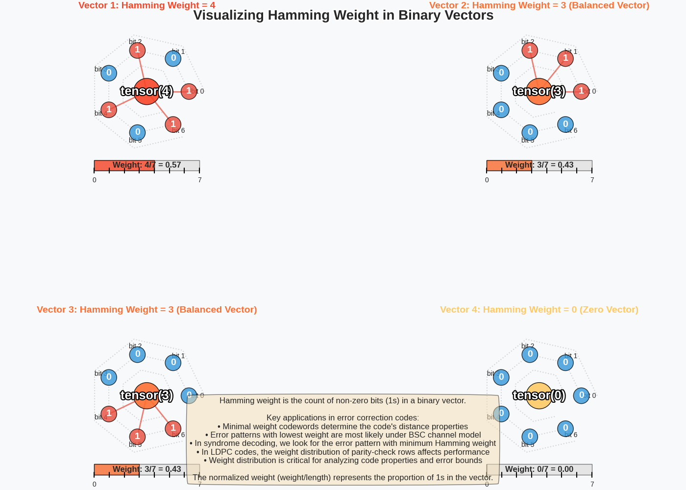
The Hamming weight is the number of non-zero elements in a binary vector, which is useful in FEC to determine the number of 1s in a codeword or error pattern.

# Create some binary vectors
vectors = [
    torch.tensor([1, 0, 1, 0, 1, 0, 1]),  # 4 ones
    torch.tensor([1, 1, 1, 0, 0, 0, 0]),  # 3 ones
    torch.tensor([0, 0, 0, 0, 1, 1, 1]),  # 3 ones
    torch.tensor([0, 0, 0, 0, 0, 0, 0]),  # 0 ones
]

for i, vec in enumerate(vectors):
    weight = hamming_weight(vec)
    print(f"Vector {i+1}: {vec}, Hamming weight: {weight}")

Vector 1: tensor([1, 0, 1, 0, 1, 0, 1]), Hamming weight: 4
Vector 2: tensor([1, 1, 1, 0, 0, 0, 0]), Hamming weight: 3
Vector 3: tensor([0, 0, 0, 0, 1, 1, 1]), Hamming weight: 3
Vector 4: tensor([0, 0, 0, 0, 0, 0, 0]), Hamming weight: 0

Visualizing Hamming Weight with Dynamic Animations

We’ll create an enhanced visualization that dynamically shows how Hamming weight represents the number of 1s in each vector, with interactive elements and color coding.

# First, create a static visualization with improved styling
fig, axes = plt.subplots(2, 2, figsize=(14, 10), gridspec_kw={"hspace": 0.5, "wspace": 0.3}, facecolor=background_color, constrained_layout=True)
axes = axes.flatten()

# Use a modern, visually appealing color gradient
weight_colors = [plt.cm.YlOrRd(x) for x in np.linspace(0.3, 0.9, 8)]

for i, (vec, ax) in enumerate(zip(vectors, axes)):
    weight = hamming_weight(vec)

    # Set a custom background with gradient effect
    ax.set_facecolor(plt.cm.Blues(0.1))

    # Create radar-like background grid
    theta = np.linspace(0, 2 * np.pi, len(vec) + 1)[:-1]
    for r in [0.5, 0.8, 1.1]:
        ax.plot(r * np.cos(theta), r * np.sin(theta), "gray", alpha=0.3, linestyle=":")

    # Plot the binary vector in a circular arrangement for a more dynamic look
    radius = 0.8
    x_pos = np.cos(theta) * radius
    y_pos = np.sin(theta) * radius

    # Draw connecting lines to center
    for j, bit in enumerate(vec):
        if bit == 1:
            # Draw a line connecting each '1' bit to the center to visualize contribution to weight
            ax.plot([0, x_pos[j]], [0, y_pos[j]], color=bit_1_color, alpha=0.7, linewidth=2, zorder=5)

    # Add circular nodes for bits
    for j, bit in enumerate(vec):
        # Choose color based on bit value (1 or 0)
        color = bit_1_color if bit == 1 else bit_0_color
        # Create a circular node for each bit in the vector
        circle = plt.Circle((x_pos[j], y_pos[j]), 0.15, facecolor=color, alpha=0.8, edgecolor="black", zorder=10)
        ax.add_patch(circle)
        # Add the bit value text in the center of each node
        ax.text(x_pos[j], y_pos[j], str(int(bit)), ha="center", va="center", fontweight="bold", fontsize=14, color="white", zorder=15)

        # Add bit position labels
        label_x = 1.2 * radius * np.cos(theta[j])
        label_y = 1.2 * radius * np.sin(theta[j])
        ax.text(label_x, label_y, f"bit {j}", ha="center", va="center", fontsize=10)

    # Create a center weighted node showing the Hamming weight
    weight_index = int(weight)  # Convert to int for indexing
    # Create a circle at the center showing the Hamming weight with color indicating magnitude
    center_circle = plt.Circle((0, 0), 0.25, facecolor=weight_colors[weight_index], alpha=0.9, edgecolor="black", zorder=20)
    ax.add_patch(center_circle)
    # Add the weight value text in the center
    ax.text(0, 0, str(weight), ha="center", va="center", fontweight="bold", fontsize=18, color="white", zorder=25, path_effects=[PathEffects.withStroke(linewidth=3, foreground="black")])

    # Add a weight meter at the bottom
    meter_width = weight / len(vec)
    # Create a background rectangle for the meter
    ax.add_patch(Rectangle((-1, -1.5), 2, 0.2, facecolor="lightgray", alpha=0.5, edgecolor="black"))
    # Create a foreground rectangle with width proportional to the weight ratio
    ax.add_patch(Rectangle((-1, -1.5), 2 * meter_width, 0.2, facecolor=weight_colors[int(weight)], alpha=0.8, edgecolor="black"))

    # Add a text label showing weight as fraction and decimal
    ax.text(0, -1.4, f"Weight: {weight}/{len(vec)} = {weight/len(vec):.2f}", ha="center", va="center", fontsize=12, fontweight="bold")

    # Scale markers
    for j in range(len(vec) + 1):
        x_mark = -1 + 2 * j / len(vec)
        ax.plot([x_mark, x_mark], [-1.55, -1.45], color="black")
        if j in [0, len(vec)]:
            ax.text(x_mark, -1.62, str(j), ha="center", va="top", fontsize=10)

    # Set a descriptive title
    title = f"Vector {i+1}: Hamming Weight = {weight}"
    if weight == 0:
        title += " (Zero Vector)"
    elif weight == len(vec):
        title += " (All Ones)"
    elif weight == len(vec) // 2:
        title += " (Balanced Vector)"

    ax.set_title(title, fontsize=14, fontweight="bold", color=weight_colors[int(weight)])

    # Set axis limits and remove ticks
    ax.set_xlim(-1.5, 1.5)
    ax.set_ylim(-1.7, 1.5)
    ax.set_aspect("equal")
    ax.axis("off")

# Add a title for the entire figure
title = fig.suptitle("Visualizing Hamming Weight in Binary Vectors", fontsize=20, fontweight="bold", y=0.98)
title.set_path_effects([PathEffects.withStroke(linewidth=4, foreground="white")])

# Add an enhanced explanation of Hamming weight
explanation = """Hamming weight is the count of non-zero bits (1s) in a binary vector.

Key applications in error correction codes:
• Minimal weight codewords determine the code's distance properties
• Error patterns with lowest weight are most likely under BSC channel model
• In syndrome decoding, we look for the error pattern with minimum Hamming weight
• In LDPC codes, the weight distribution of parity-check rows affects performance
• Weight distribution is critical for analyzing code properties and error bounds

The normalized weight (weight/length) represents the proportion of 1s in the vector."""

fig.text(0.5, 0.02, explanation, ha="center", fontsize=12, bbox=dict(boxstyle="round4,pad=0.5", facecolor="wheat", alpha=0.5))

plt.show()

Binary-Integer Conversions

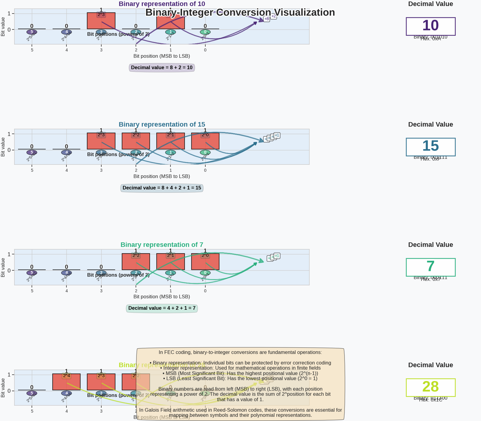
In FEC coding, we often need to convert between binary and integer representations. The utility functions to_binary_tensor and from_binary_tensor help with this.

# Convert integers to binary tensors
integers = [10, 15, 7, 28]
binary_length = 6  # Length of binary representation

binary_tensors = [to_binary_tensor(x, binary_length) for x in integers]

# Display the conversions
for i, num in enumerate(integers):
    bin_tensor = binary_tensors[i]
    print(f"Integer: {num}, Binary: {bin_tensor}")

    # Verify the conversion back to integer
    int_back = from_binary_tensor(bin_tensor)
    print(f"Converted back: {int_back}")
    print()

Integer: 10, Binary: tensor([0, 0, 1, 0, 1, 0], dtype=torch.int32)
Converted back: 10

Integer: 15, Binary: tensor([0, 0, 1, 1, 1, 1], dtype=torch.int32)
Converted back: 15

Integer: 7, Binary: tensor([0, 0, 0, 1, 1, 1], dtype=torch.int32)
Converted back: 7

Integer: 28, Binary: tensor([0, 1, 1, 1, 0, 0], dtype=torch.int32)
Converted back: 28

Visualizing Binary-Integer Conversions with Interactive Elements

Let’s create a more informative and visually appealing visualization showing the relationship between binary and decimal representations.

fig = plt.figure(figsize=(16, 14), facecolor=background_color, constrained_layout=True)
gs = GridSpec(len(integers), 2, width_ratios=[3, 1], wspace=0.3, hspace=0.6, figure=fig)

# Create a transition effect between panels
transition_colors = plt.cm.viridis(np.linspace(0.1, 0.9, len(integers)))

for i, num in enumerate(integers):
    binary = binary_tensors[i].numpy()

    # Plot the binary representation with 3D effect
    ax_bin = fig.add_subplot(gs[i, 0], facecolor=plt.cm.Blues(0.1))

    # Calculate positional values
    positions = np.arange(len(binary))
    values = [2 ** (len(binary) - j - 1) if binary[j] == 1 else 0 for j in range(len(binary))]

    # Create the bar chart with enhanced styling
    bars = ax_bin.bar(positions, binary, color=[bit_1_color if bit == 1 else bit_0_color for bit in binary], edgecolor="black", linewidth=1.5, alpha=0.8, bottom=0.05)  # Add a small bottom for 3D effect

    # Add bit value labels with enhanced styling
    for j, bit in enumerate(binary):
        txt = ax_bin.text(j, bit + 0.1, str(int(bit)), ha="center", fontweight="bold", fontsize=14)
        txt.set_path_effects([PathEffects.withStroke(linewidth=2, foreground="white")])

    # Add positional value indicators with better styling
    for j, (bit, val) in enumerate(zip(binary, values)):
        # Position in binary
        pos_val = 2 ** (len(binary) - j - 1)

        # For bits with value 1, add value indicators
        if bit == 1:
            # Add flowing arrow to show contribution
            arrow = FancyArrowPatch((j, bit / 2), (len(binary) + 0.5, 0.5), connectionstyle=f"arc3,rad={0.2 + j*0.05}", arrowstyle="fancy,head_length=6,head_width=6", color=transition_colors[i], linewidth=2, alpha=0.7, zorder=5)
            ax_bin.add_patch(arrow)

            # Add value contribution text
            ax_bin.text(j, bit - 0.15, f"2^{len(binary)-j-1}", ha="center", fontsize=11, color="black", bbox=dict(boxstyle="round,pad=0.2", facecolor=transition_colors[i], alpha=0.2))

            # Add value at the end of the arrow
            ax_bin.text(len(binary) + 0.5 + j * 0.1, 0.5 + j * 0.08, f"+{pos_val}", ha="left", va="center", fontsize=10, color=transition_colors[i], bbox=dict(boxstyle="round,pad=0.2", facecolor="white", alpha=0.7))

    # Add bit position indicators with better styling
    ax_bin.text(len(binary) / 2 - 0.5, -0.3, "Bit positions (powers of 2)", ha="center", va="center", fontsize=12, fontweight="bold")

    for j in range(len(binary)):
        pos_circle = CirclePolygon((j, -0.15), 0.15, resolution=20, facecolor=modern_palette[j % len(modern_palette)], alpha=0.7, edgecolor="black")
        ax_bin.add_patch(pos_circle)
        ax_bin.text(j, -0.15, f"{len(binary)-j-1}", ha="center", va="center", fontweight="bold", fontsize=10, color="white")

        # Add the value of each position
        ax_bin.text(j, -0.4, f"2^{len(binary)-j-1}={2**(len(binary)-j-1)}", ha="center", va="center", fontsize=9, rotation=45)

    # Add a formula showing the conversion calculation with animation-like styling
    terms = [f"{2**(len(binary)-j-1)}" for j, bit in enumerate(binary) if bit == 1]
    if terms:
        formula = " + ".join(terms)

        # Add mathematical representation
        formula_box = ax_bin.text(0.5, -0.7, f"Decimal value = {formula} = {num}", transform=ax_bin.transAxes, ha="center", fontsize=12, fontweight="bold", color="black", bbox=dict(boxstyle="round4,pad=0.5", facecolor=transition_colors[i], alpha=0.2))
    else:
        # Special case for zero
        formula_box = ax_bin.text(0.5, -0.7, "Decimal value = 0", transform=ax_bin.transAxes, ha="center", fontsize=12, fontweight="bold", color="black", bbox=dict(boxstyle="round4,pad=0.5", facecolor=transition_colors[i], alpha=0.2))

    # Add connecting line to decimal value
    arrow = FancyArrowPatch((len(binary) / 2, -0.9), (len(binary) + 0.7, 0.5), connectionstyle="arc3,rad=-0.3", arrowstyle="fancy,head_length=10,head_width=10", color=transition_colors[i], linewidth=2.5, zorder=5, alpha=0.7)
    ax_bin.add_patch(arrow)

    ax_bin.set_title(f"Binary representation of {num}", fontsize=16, fontweight="bold", color=transition_colors[i])
    ax_bin.set_xlabel("Bit position (MSB to LSB)", fontsize=12)
    ax_bin.set_ylabel("Bit value", fontsize=12)
    ax_bin.set_yticks([0, 1])
    ax_bin.set_xticks(positions)
    ax_bin.set_xticklabels([f"{len(binary)-j-1}" for j in positions], fontsize=10)
    ax_bin.set_ylim(-0.9, 1.3)
    ax_bin.set_xlim(-0.5, len(binary) + 2)

    # Plot the decimal representation with enhanced styling
    ax_dec = fig.add_subplot(gs[i, 1], facecolor=plt.cm.Blues(0.1))

    # Create a fancy decimal display
    decimal_box = Rectangle((0.25, 0.25), 0.5, 0.5, linewidth=2, edgecolor=transition_colors[i], facecolor="white", alpha=0.9, zorder=5)
    ax_dec.add_patch(decimal_box)

    # Add the decimal value with glow effect
    txt = ax_dec.text(0.5, 0.5, str(num), ha="center", va="center", fontsize=36, fontweight="bold", color=transition_colors[i], zorder=10)
    txt.set_path_effects([PathEffects.withStroke(linewidth=5, foreground="white")])

    # Add binary representation below
    binary_str = "".join([str(int(b)) for b in binary])
    ax_dec.text(0.5, 0.2, f"Binary: {binary_str}", ha="center", va="center", fontsize=12, transform=ax_dec.transAxes)

    # Add hexadecimal representation
    ax_dec.text(0.5, 0.15, f"Hex: 0x{num:X}", ha="center", va="center", fontsize=12, transform=ax_dec.transAxes)

    ax_dec.set_title("Decimal Value", fontsize=16, fontweight="bold")
    ax_dec.axis("off")

# Add a title for the entire figure with enhanced styling
title = fig.suptitle("Binary-Integer Conversion Visualization", fontsize=24, fontweight="bold", y=0.98)
title.set_path_effects([PathEffects.withStroke(linewidth=4, foreground="white")])

# Add enhanced explanation
explanation = """In FEC coding, binary-to-integer conversions are fundamental operations:

• Binary representation: Individual bits can be protected by error correction coding
• Integer representation: Used for mathematical operations in finite fields
• MSB (Most Significant Bit): Has the highest positional value (2^(n-1))
• LSB (Least Significant Bit): Has the lowest positional value (2^0 = 1)

Binary numbers are read from left (MSB) to right (LSB), with each position
representing a power of 2. The decimal value is the sum of 2^position for each bit
that has a value of 1.

In Galois Field arithmetic used in Reed-Solomon codes, these conversions are essential for
mapping between symbols and their polynomial representations."""

fig.text(0.5, 0.01, explanation, ha="center", fontsize=12, bbox=dict(boxstyle="round4,pad=0.7", facecolor="wheat", alpha=0.6))

plt.show()

3D Visualization of Hamming Distance Relationships

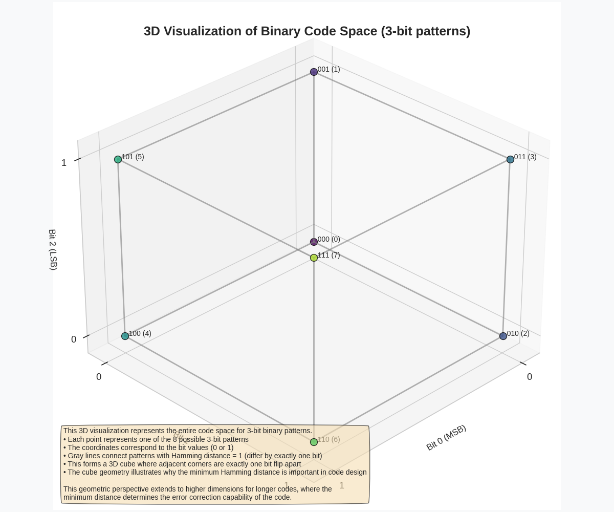
Let’s create a 3D visualization showing the Hamming distance relationships between different binary patterns, creating a geometric perspective of the code space.

# Create 3-bit binary patterns (8 possible patterns)
patterns = []
for i in range(8):
    patterns.append(to_binary_tensor(i, 3))

# Calculate pairwise Hamming distances
distances = np.zeros((len(patterns), len(patterns)))
for i in range(len(patterns)):
    for j in range(len(patterns)):
        distances[i, j] = hamming_distance(patterns[i], patterns[j])

# Create 3D coordinates for each pattern based on their bits
coordinates = np.array([[int(b) for b in p] for p in patterns])

# Set up the 3D plot with constrained layout
fig = plt.figure(figsize=(12, 10), facecolor=background_color, constrained_layout=True)
ax = fig.add_subplot(111, projection="3d")

# Plot each point (binary pattern)
for i, coord in enumerate(coordinates):
    ax.scatter(coord[0], coord[1], coord[2], color=plt.cm.viridis(i / len(patterns)), s=100, edgecolor="black", alpha=0.8)

    # Add binary label
    binary_str = "".join([str(int(b)) for b in patterns[i]])
    ax.text(coord[0], coord[1], coord[2], f"  {binary_str} ({from_binary_tensor(patterns[i])})", fontsize=10)

# Draw edges between patterns with Hamming distance 1
for i in range(len(patterns)):
    for j in range(i + 1, len(patterns)):
        if distances[i, j] == 1:
            ax.plot([coordinates[i, 0], coordinates[j, 0]], [coordinates[i, 1], coordinates[j, 1]], [coordinates[i, 2], coordinates[j, 2]], color="gray", alpha=0.6, linewidth=2)

# Customize the appearance
ax.set_xlabel("Bit 0 (MSB)", fontsize=12)
ax.set_ylabel("Bit 1", fontsize=12)
ax.set_zlabel("Bit 2 (LSB)", fontsize=12)
ax.set_xlim(-0.1, 1.1)
ax.set_ylim(-0.1, 1.1)
ax.set_zlim(-0.1, 1.1)
ax.set_xticks([0, 1])
ax.set_yticks([0, 1])
ax.set_zticks([0, 1])
ax.view_init(elev=30, azim=45)  # Set initial viewing angle

# Add title and explanation
title = fig.suptitle("3D Visualization of Binary Code Space (3-bit patterns)", fontsize=18, fontweight="bold", y=0.95)
title.set_path_effects([PathEffects.withStroke(linewidth=4, foreground="white")])

explanation = """This 3D visualization represents the entire code space for 3-bit binary patterns.
• Each point represents one of the 8 possible 3-bit patterns
• The coordinates correspond to the bit values (0 or 1)
• Gray lines connect patterns with Hamming distance = 1 (differ by exactly one bit)
• This forms a 3D cube where adjacent corners are exactly one bit flip apart
• The cube geometry illustrates why the minimum Hamming distance is important in code design

This geometric perspective extends to higher dimensions for longer codes, where the
minimum distance determines the error correction capability of the code."""

ax.text2D(0.02, 0.02, explanation, transform=ax.transAxes, fontsize=10, bbox=dict(boxstyle="round4,pad=0.5", facecolor="wheat", alpha=0.6))

plt.show()

Conclusion

In this example, we’ve explored fundamental binary operations used in forward error correction (FEC) coding with enhanced visualizations:

Key points: - Hamming distance quantifies differences between binary sequences, which directly determines error detection and correction capabilities - Hamming weight counts the number of 1s in a binary sequence, crucial for analyzing code properties and error patterns - Binary-integer conversions are essential for implementing FEC algorithms and working with finite field arithmetic

These basic operations form the foundation for more advanced FEC techniques like Hamming codes, Reed-Solomon codes, and LDPC codes. The 3D geometric visualization helps build intuition about how code space relates to error correction.

References: - [Lin and Costello, 2004] - Provides comprehensive coverage of error control coding - [Moon, 2005] - Explains mathematical methods for error correction - [MacWilliams and Sloane, 1977] - Classic text on the theory of error-correcting codes