Note
Go to the end to download the full example code. or to run this example in your browser via Binder
Discrete Task-Oriented Deep JSCC Model (Xie 2023)
This example demonstrates how to use the Discrete Task-Oriented Deep JSCC (DT-DeepJSCC) model from Xie et al. (2023). Unlike traditional DeepJSCC which focuses on image reconstruction, DT-DeepJSCC is designed for task-oriented semantic communications, specifically for image classification tasks. It uses a discrete bottleneck for robustness against channel impairments.
import matplotlib.pyplot as plt
import numpy as np
import torch
import torch.nn.functional as F

from kaira.channels import AWGNChannel, BinarySymmetricChannel
from kaira.constraints import TotalPowerConstraint
from kaira.data.sample_data import load_sample_images
from kaira.models.deepjscc import DeepJSCCModel
from kaira.models.image.xie2023_dt_deepjscc import (
    Xie2023DTDeepJSCCDecoder,
    Xie2023DTDeepJSCCEncoder,
)

# Set random seed for reproducibility
torch.manual_seed(42)
np.random.seed(42)
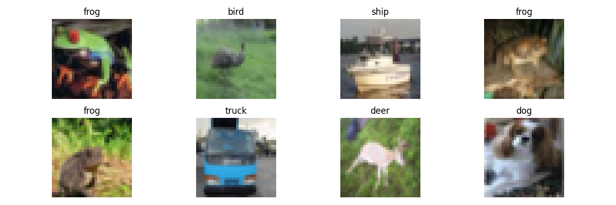
Loading Sample Images
We’ll use sample images for our task-oriented semantic communication example
# Load sample images
sample_images, sample_labels = load_sample_images(dataset="cifar10", num_samples=8, seed=42)
sample_batch_size = 8  # Number of samples to visualize

# Class names for CIFAR-10
class_names = ["airplane", "automobile", "bird", "cat", "deer", "dog", "frog", "horse", "ship", "truck"]

# Display sample images
plt.figure(figsize=(12, 4))
for i in range(sample_batch_size):
    plt.subplot(2, 4, i + 1)
    plt.imshow(sample_images[i].permute(1, 2, 0).numpy())
    plt.title(f"{class_names[sample_labels[i]]}")
    plt.axis("off")
plt.tight_layout()
Creating the DT-DeepJSCC Model
Construct the Discrete Task-Oriented DeepJSCC model for semantic image classification
# Define model parameters
in_channels = 3  # RGB images
latent_channels = 64  # Dimension of latent representation
out_classes = 10  # CIFAR-10 has 10 classes
architecture = "cifar10"  # Using architecture optimized for CIFAR-10 images
num_embeddings = 400  # Size of discrete codebook

# Create the encoder and decoder components
encoder = Xie2023DTDeepJSCCEncoder(in_channels=in_channels, latent_channels=latent_channels, architecture=architecture, num_embeddings=num_embeddings)

decoder = Xie2023DTDeepJSCCDecoder(latent_channels=latent_channels, out_classes=out_classes, architecture=architecture, num_embeddings=num_embeddings)

# Set up power constraint and channel
power_constraint = TotalPowerConstraint(total_power=1.0)
channel = AWGNChannel(snr_db=10)  # Default SNR value

# Create the complete DeepJSCC model
model = DeepJSCCModel(encoder=encoder, constraint=power_constraint, channel=channel, decoder=decoder)

print("DT-DeepJSCC Model Configuration:")
print(f"- Architecture: {architecture}")
print(f"- Input channels: {in_channels}")
print(f"- Latent channels: {latent_channels}")
print(f"- Output classes: {out_classes}")
print(f"- Codebook size: {num_embeddings}")
print(f"- Bits per symbol: {int(np.log2(num_embeddings))}")
DT-DeepJSCC Model Configuration:
- Architecture: cifar10
- Input channels: 3
- Latent channels: 64
- Output classes: 10
- Codebook size: 400
- Bits per symbol: 8
Testing Classification Performance Over Different Channels
Let’s compare how the model performs over different channel types and conditions
def evaluate_classification(model, images, labels, snr=None):
    """Evaluate model classification performance."""
    with torch.no_grad():
        # Update the channel's SNR if provided
        if snr is not None:
            model.channel.snr_db = snr

        # Pass images through the model
        logits = model(images)

        # Get predictions
        predictions = torch.argmax(logits, dim=1)

        # Calculate accuracy
        accuracy = (predictions == labels).float().mean().item()

        return accuracy, predictions


# Test across different SNR values for AWGN channel
snr_values = [0, 5, 10, 15, 20]
awgn_accuracies = []

for snr in snr_values:
    accuracy, _ = evaluate_classification(model, sample_images, sample_labels, snr=snr)
    awgn_accuracies.append(accuracy)
    print(f"AWGN Channel - SNR: {snr} dB, Accuracy: {accuracy:.4f}")

# Test with Binary Symmetric Channel at different bit flip probabilities
# First save the original channel
original_channel = model.channel

# Create BSC channel and test
bsc_flip_probs = [0.001, 0.01, 0.05, 0.1, 0.2]
bsc_accuracies = []

for p in bsc_flip_probs:
    # Set BSC channel
    model.channel = BinarySymmetricChannel(crossover_prob=p)

    # Evaluate
    accuracy, _ = evaluate_classification(model, sample_images, sample_labels)
    bsc_accuracies.append(accuracy)
    print(f"BSC Channel - Bit flip prob: {p}, Accuracy: {accuracy:.4f}")

# Restore original channel
model.channel = original_channel
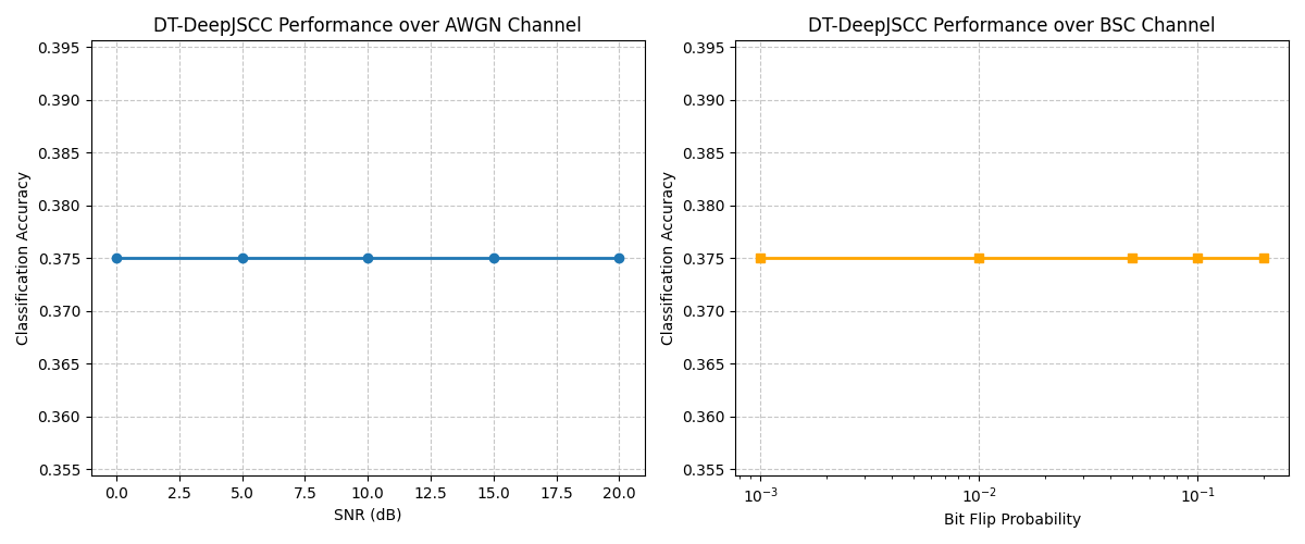
AWGN Channel - SNR: 0 dB, Accuracy: 0.3750
AWGN Channel - SNR: 5 dB, Accuracy: 0.3750
AWGN Channel - SNR: 10 dB, Accuracy: 0.3750
AWGN Channel - SNR: 15 dB, Accuracy: 0.3750
AWGN Channel - SNR: 20 dB, Accuracy: 0.3750
BSC Channel - Bit flip prob: 0.001, Accuracy: 0.3750
BSC Channel - Bit flip prob: 0.01, Accuracy: 0.3750
BSC Channel - Bit flip prob: 0.05, Accuracy: 0.3750
BSC Channel - Bit flip prob: 0.1, Accuracy: 0.3750
BSC Channel - Bit flip prob: 0.2, Accuracy: 0.3750
Visualizing Results with Different Channel Conditions
Visualize classification performance across different channel conditions
# Plot accuracy vs SNR for AWGN
plt.figure(figsize=(12, 5))

# AWGN results
plt.subplot(1, 2, 1)
plt.plot(snr_values, awgn_accuracies, "o-", linewidth=2)
plt.grid(True, linestyle="--", alpha=0.7)
plt.xlabel("SNR (dB)")
plt.ylabel("Classification Accuracy")
plt.title("DT-DeepJSCC Performance over AWGN Channel")

# BSC results
plt.subplot(1, 2, 2)
plt.plot(bsc_flip_probs, bsc_accuracies, "s-", linewidth=2, color="orange")
plt.grid(True, linestyle="--", alpha=0.7)
plt.xlabel("Bit Flip Probability")
plt.ylabel("Classification Accuracy")
plt.title("DT-DeepJSCC Performance over BSC Channel")
plt.xscale("log")  # Log scale for better visualization

plt.tight_layout()
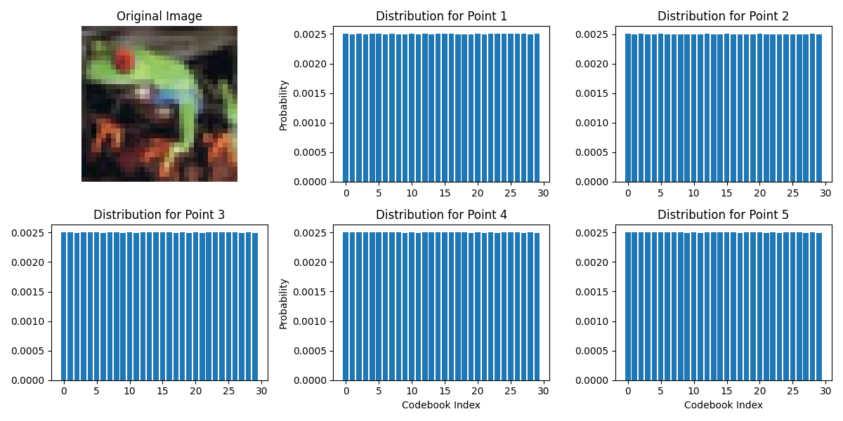
Understanding the Discrete Bottleneck
Visualize how the discrete bottleneck works in practice
# Create a simplified view of the discrete bottleneck process
plt.figure(figsize=(12, 6))


# Function to show the discrete bottleneck process
def visualize_discrete_bottleneck(image, indices=None):
    """Process an image through the discrete bottleneck of the encoder to visualize how the
    discrete representation works.

    This function performs a forward pass through the encoder to obtain feature
    representations, applies the discrete bottleneck, and returns various
    intermediate representations for visualization purposes.

    Parameters
    ----------
    image : torch.Tensor
        The input image tensor with shape [C, H, W]
    indices : torch.Tensor, optional
        Pre-computed indices if available, by default None

    Returns
    -------
    tuple
        A tuple containing:
        - features (torch.Tensor): The feature representation before bottleneck
        - indices (torch.Tensor): The discrete indices selected from the codebook
        - dist (torch.Tensor): The distribution over codebook indices
        - one_hot (torch.Tensor): One-hot encoding of the selected indices
    """
    # Forward pass through encoder (without channel)
    with torch.no_grad():
        # Get features before bottleneck
        features = encoder.encoder(image.unsqueeze(0))

        # Reshape features to apply the discrete bottleneck
        if encoder.is_convolutional:
            b, c, h, w = features.shape
            features_reshaped = features.permute(0, 2, 3, 1).contiguous()
            features_reshaped = features_reshaped.view(-1, encoder.latent_d)
        else:
            features_reshaped = features.view(1, -1)

        # Get indices and distribution
        indices, dist = encoder.sampler(features_reshaped)

        # Get one-hot encoding of indices
        one_hot = F.one_hot(indices, num_classes=encoder.num_embeddings).float()

        return features, indices, dist, one_hot


# Use our test image
test_img = sample_images[0]
features, indices, dist, one_hot = visualize_discrete_bottleneck(test_img)

# Plot the first n_samples codebook distributions for this image
n_samples = 6
plt.subplot(2, 3, 1)
plt.imshow(test_img.permute(1, 2, 0).numpy())
plt.title("Original Image")
plt.axis("off")

# Plot distribution over codebook for a few selected points
dist_size = dist.size(0)
stride = max(1, dist_size // 5)  # Ensure we select at most 5 well-spaced points

for i in range(min(5, n_samples)):
    idx = min(i * stride, dist_size - 1)  # Ensure index is within bounds
    plt.subplot(2, 3, i + 2)
    plt.bar(range(min(30, encoder.num_embeddings)), dist[idx][: min(30, encoder.num_embeddings)].cpu().numpy())
    plt.title(f"Distribution for Point {i+1}")
    plt.xlabel("Codebook Index" if i >= 3 else "")
    plt.ylabel("Probability" if i % 3 == 0 else "")

plt.tight_layout()
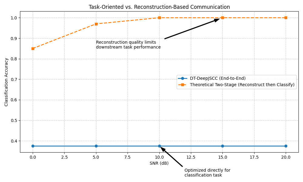
Comparing with Standard DeepJSCC Performance
Conceptual comparison between task-oriented and reconstruction-based DeepJSCC
# Theoretical performance data for comparison
snr_range = np.array(snr_values)
classification_accuracy = np.array(awgn_accuracies)

# Theoretical PSNR values for a standard DeepJSCC model (for comparison)
theoretical_psnr = 15 + 0.8 * snr_range  # Hypothetical PSNR scaling with SNR

# Theoretical accuracy of a two-stage system (reconstruct then classify)
theoretical_two_stage = 0.4 + 0.03 * theoretical_psnr  # Hypothetical accuracy scaling with PSNR
theoretical_two_stage = np.clip(theoretical_two_stage, 0, 1)

plt.figure(figsize=(10, 6))
plt.plot(snr_range, classification_accuracy, "o-", linewidth=2, label="DT-DeepJSCC (End-to-End)")
plt.plot(snr_range, theoretical_two_stage, "s--", linewidth=2, label="Theoretical Two-Stage (Reconstruct then Classify)")

plt.grid(True, linestyle="--", alpha=0.7)
plt.xlabel("SNR (dB)")
plt.ylabel("Classification Accuracy")
plt.title("Task-Oriented vs. Reconstruction-Based Communication")
plt.legend()

# Add annotations explaining the key differences
plt.annotate("Optimized directly for\nclassification task", xy=(10, classification_accuracy[2]), xytext=(12, classification_accuracy[2] - 0.15), arrowprops=dict(facecolor="black", shrink=0.05, width=1.5, headwidth=8))

plt.annotate("Reconstruction quality limits\ndownstream task performance", xy=(15, theoretical_two_stage[3]), xytext=(5, theoretical_two_stage[3] - 0.15), arrowprops=dict(facecolor="black", shrink=0.05, width=1.5, headwidth=8))

plt.tight_layout()
Benefits of Discrete Task-Oriented DeepJSCC
Key advantages of the DT-DeepJSCC approach:
Task Optimization: The model is optimized directly for classification rather than reconstruction, leading to better performance on the specific task.
Discrete Bottleneck: The discrete representation provides robustness against channel noise and allows for better quantization.
Bandwidth Efficiency: The model can achieve good classification performance at lower bit rates compared to reconstruction-based approaches.
Channel Adaptability: Performance degrades gracefully across different channel conditions, as shown in our experiments.
References: - Original paper: [Xie et al., 2023] - GitHub repository: https://github.com/SongjieXie/Discrete-TaskOriented-JSCC
Visualizing the Modulation, Channel, and Demodulation Pipeline
Let’s visualize the end-to-end communication pipeline with modulation, channel effects, and demodulation
print("\nExploring DT-DeepJSCC Communication Pipeline:")
print("=============================================")


# Function to demonstrate the full pipeline for an image
def demonstrate_communication_pipeline(model, image, snr_db=10):
    """Demonstrate the full communication pipeline from image to classification."""
    with torch.no_grad():
        # Step 1: Encoding (includes modulation)
        print("Step 1: Image Encoding & Modulation")
        # Get the encoded representation
        encoded = model.encoder(image.unsqueeze(0))

        # Extract modulated symbols (after power constraint)
        modulated = model.constraint(encoded)

        # Step 2: Channel Transmission
        print("Step 2: Channel Transmission")
        # Set channel SNR
        model.channel.snr_db = snr_db
        print(f"- Channel: {model.channel.__class__.__name__}")
        print(f"- SNR: {snr_db} dB")

        # Pass through channel
        received = model.channel(modulated)

        # Step 3: Decoding (includes demodulation)
        print("Step 3: Demodulation & Decoding")
        decoded = model.decoder(received)

        # Get prediction
        prediction = torch.argmax(decoded, dim=1).item()

        # Return intermediate representations for visualization
        return {"encoded": encoded.detach(), "modulated": modulated.detach(), "received": received.detach(), "decoded": decoded.detach(), "prediction": prediction}


# Demonstrate the pipeline for a sample image
test_image = sample_images[3]  # Choose a sample image
test_label = sample_labels[3]
results = demonstrate_communication_pipeline(model, test_image, snr_db=15)

print(f"\nInput image class: {class_names[test_label]}")
print(f"Predicted class: {class_names[results['prediction']]}")

# Visualize the original image and modulated signal
plt.figure(figsize=(15, 8))

# Original image
plt.subplot(2, 2, 1)
plt.imshow(test_image.permute(1, 2, 0).numpy())
plt.title(f"Original Image: {class_names[test_label]}")
plt.axis("off")

# Modulated signal (take first few dimensions to visualize)
modulated_data = results["modulated"][0].cpu().numpy()

# For stem plot, use only the first dimension if it's multi-dimensional
if len(modulated_data.shape) > 1:
    # Extract just the first 16 values from the first dimension
    plot_data = modulated_data[0, :16]
    signal_length = len(plot_data)
else:
    # If it's already 1D, take first 16 values
    plot_data = modulated_data[:16]
    signal_length = len(plot_data)

plt.subplot(2, 2, 2)
# Use the prepared data directly
plt.stem(range(signal_length), plot_data)
plt.title("Modulated Signal (First 16 symbols)")
plt.xlabel("Symbol Index")
plt.ylabel("Amplitude")
plt.grid(True, alpha=0.3)

# Show received signal (with channel effects)
received_data = results["received"][0].cpu().numpy()

# For stem plot, use only the first dimension if it's multi-dimensional
if len(received_data.shape) > 1:
    # Extract just the first 16 values from the first dimension
    received_plot_data = received_data[0, :16]
    received_length = len(received_plot_data)
else:
    # If it's already 1D, take first 16 values
    received_plot_data = received_data[:16]
    received_length = len(received_plot_data)

plt.subplot(2, 2, 3)
# Use the prepared data directly
plt.stem(range(received_length), received_plot_data, linefmt="r-")
plt.title(f"Received Signal (After {model.channel.__class__.__name__})")
plt.xlabel("Symbol Index")
plt.ylabel("Amplitude")
plt.grid(True, alpha=0.3)

# Visualize decoder output (class probabilities)
class_probs = F.softmax(results["decoded"][0], dim=0).cpu().numpy()

plt.subplot(2, 2, 4)
plt.bar(range(len(class_names)), class_probs)
plt.xticks(range(len(class_names)), class_names, rotation=45)
plt.title(f"Decoded Classification Probabilities\nPrediction: {class_names[results['prediction']]}")
plt.ylabel("Probability")
plt.grid(True, axis="y", alpha=0.3)

plt.tight_layout()
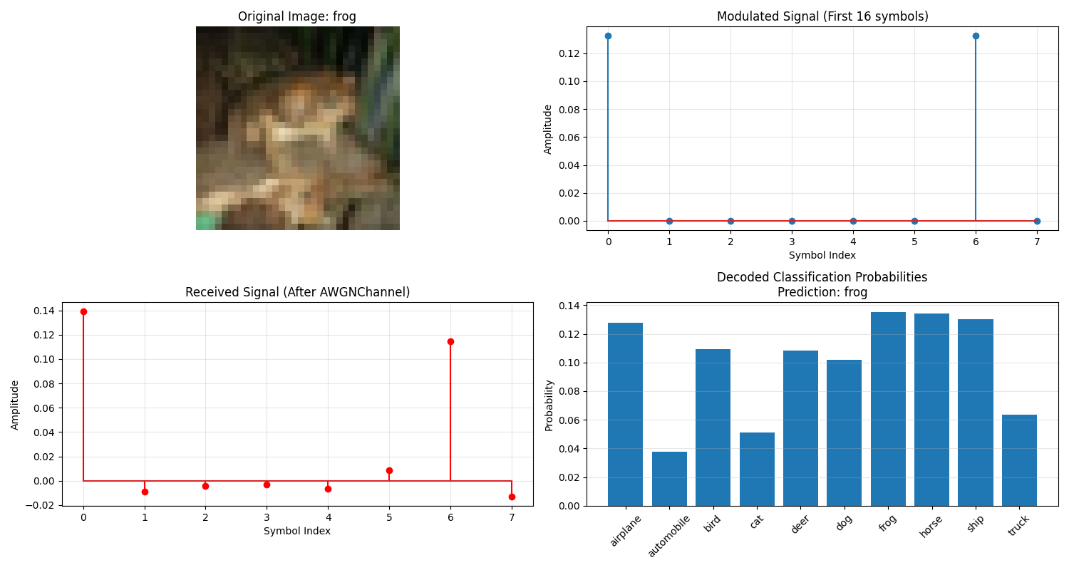
Exploring DT-DeepJSCC Communication Pipeline:
=============================================
Step 1: Image Encoding & Modulation
Step 2: Channel Transmission
- Channel: AWGNChannel
- SNR: 15 dB
Step 3: Demodulation & Decoding

Input image class: frog
Predicted class: frog
Channel Impact on Modulated Signal
Visualize how different channel conditions affect the modulated signal
# Setup for comparison
test_snrs = [5, 15, 25]
original_channel = model.channel
comparison_results = []

# Create two separate figures to avoid exceeding subplot limits
plt.figure(figsize=(15, 5))

# Show original image
plt.subplot(1, 4, 1)
plt.imshow(test_image.permute(1, 2, 0).numpy())
plt.title(f"Original: {class_names[test_label]}")
plt.axis("off")

# Process through multiple SNRs
for i, snr in enumerate(test_snrs):
    # Configure channel and process
    model.channel = AWGNChannel(snr_db=snr)
    results = demonstrate_communication_pipeline(model, test_image, snr_db=snr)
    comparison_results.append(results)

    # Get actual data size for modulated and received signals
    mod_data = results["modulated"][0].cpu().numpy()
    rec_data = results["received"][0].cpu().numpy()

    # For stem plot, use only the first dimension if it's multi-dimensional
    if len(rec_data.shape) > 1:
        # Extract values from the first dimension
        rec_plot_data = rec_data[0, :16]
        signal_length = len(rec_plot_data)
    else:
        # If it's already 1D, take first 16 values
        rec_plot_data = rec_data[:16]
        signal_length = len(rec_plot_data)

    # Show received signal (varies by SNR)
    plt.subplot(1, 4, i + 2)
    plt.stem(range(signal_length), rec_plot_data, linefmt="r-")
    plt.title(f"Received Signal (SNR={snr} dB)")
    plt.xlabel("Symbol Index")
    plt.ylabel("Amplitude")

plt.tight_layout()

# Create second figure for the class probabilities
plt.figure(figsize=(15, 5))
for i, snr in enumerate(test_snrs):
    results = comparison_results[i]

    # First subplot: Show classification probabilities
    plt.subplot(1, 3, i + 1)
    class_probs = F.softmax(results["decoded"][0], dim=0).cpu().numpy()

    # Bar plot for probabilities
    bars = plt.bar(range(len(class_names)), class_probs)
    plt.xticks(range(len(class_names)), class_names, rotation=90)
    plt.title(f"Classification at SNR={test_snrs[i]} dB")
    plt.ylabel("Probability")

    # Highlight the predicted class
    prediction = results["prediction"]
    if prediction == test_label:
        bars[prediction].set_color("green")
        predict_text = f"✓ Correct: {class_names[prediction]}"
    else:
        bars[prediction].set_color("red")
        predict_text = f"✗ Wrong: {class_names[prediction]}\nActual: {class_names[test_label]}"

    # Add prediction text
    plt.annotate(predict_text, xy=(0.5, 0.95), xycoords="axes fraction", ha="center", va="top", fontsize=10, bbox=dict(boxstyle="round,pad=0.3", fc="white", ec="gray", alpha=0.8))

plt.tight_layout()

# Restore original channel
model.channel = original_channel
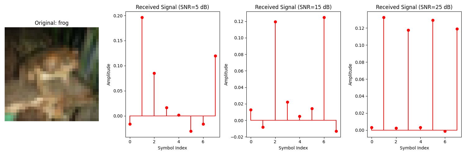
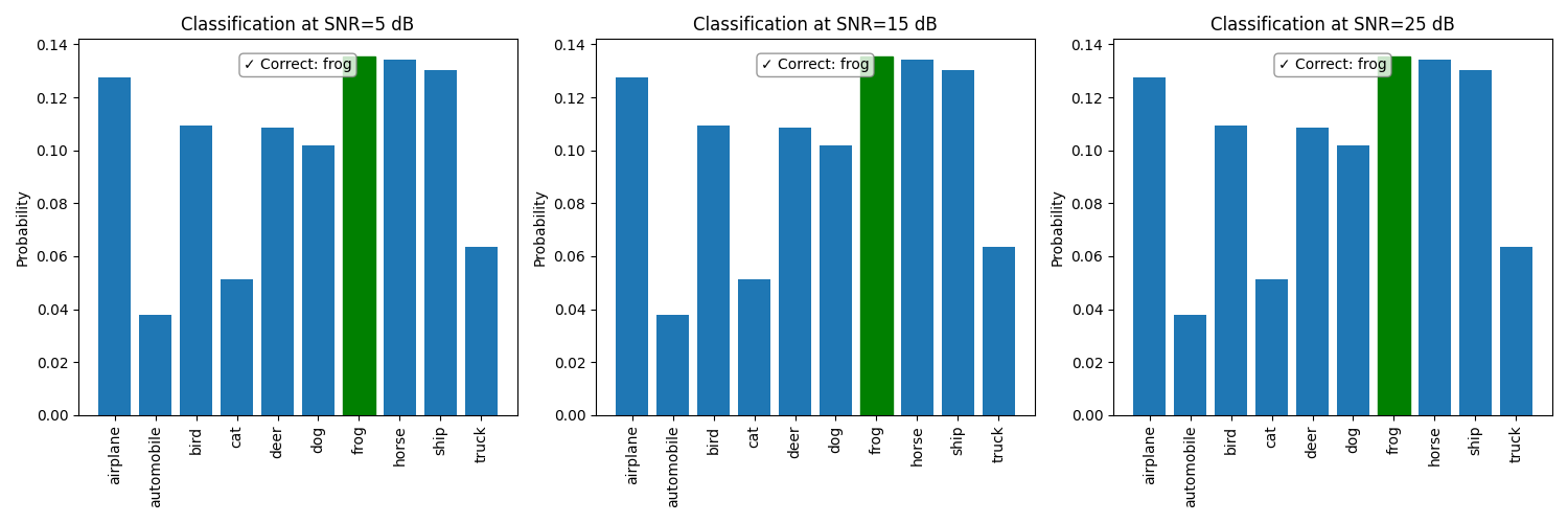
Step 1: Image Encoding & Modulation
Step 2: Channel Transmission
- Channel: AWGNChannel
- SNR: 5 dB
Step 3: Demodulation & Decoding
Step 1: Image Encoding & Modulation
Step 2: Channel Transmission
- Channel: AWGNChannel
- SNR: 15 dB
Step 3: Demodulation & Decoding
Step 1: Image Encoding & Modulation
Step 2: Channel Transmission
- Channel: AWGNChannel
- SNR: 25 dB
Step 3: Demodulation & Decoding
Comparing Different Modulation Schemes
Compare modulation through various channel conditions (AWGN vs. BSC)
# Compare performance across different channel types
plt.figure(figsize=(12, 6))

# Plot our results
plt.subplot(1, 2, 1)
plt.plot(snr_values, awgn_accuracies, "o-", linewidth=2, label="AWGN Performance")
plt.grid(True, linestyle="--", alpha=0.7)
plt.xlabel("SNR (dB)")
plt.ylabel("Classification Accuracy")
plt.ylim(0, 1.05)
plt.title("Performance over AWGN Channel")
plt.legend()

# BSC results - show traditional modulation limitations
plt.subplot(1, 2, 2)
plt.plot(bsc_flip_probs, bsc_accuracies, "s-", linewidth=2, color="orange", label="DT-DeepJSCC")

# Add theoretical curve for traditional digital system with modulation
theoretical_digital = []
for p in bsc_flip_probs:
    # In a traditional system with separate components, a high bit error rate
    # would more severely impact classification accuracy
    if p < 0.01:
        acc = 0.9  # Good performance at very low error rates
    elif p < 0.05:
        acc = 0.7  # Moderate degradation
    elif p < 0.1:
        acc = 0.4  # Severe degradation
    else:
        acc = 0.2  # Near-random performance at high error rates
    theoretical_digital.append(acc)

plt.plot(bsc_flip_probs, theoretical_digital, "d--", linewidth=2, color="green", label="Traditional Digital")

plt.grid(True, linestyle="--", alpha=0.7)
plt.xlabel("Bit Flip Probability")
plt.xscale("log")
plt.ylabel("Classification Accuracy")
plt.ylim(0, 1.05)
plt.title("Performance over BSC Channel")
plt.legend()

plt.tight_layout()
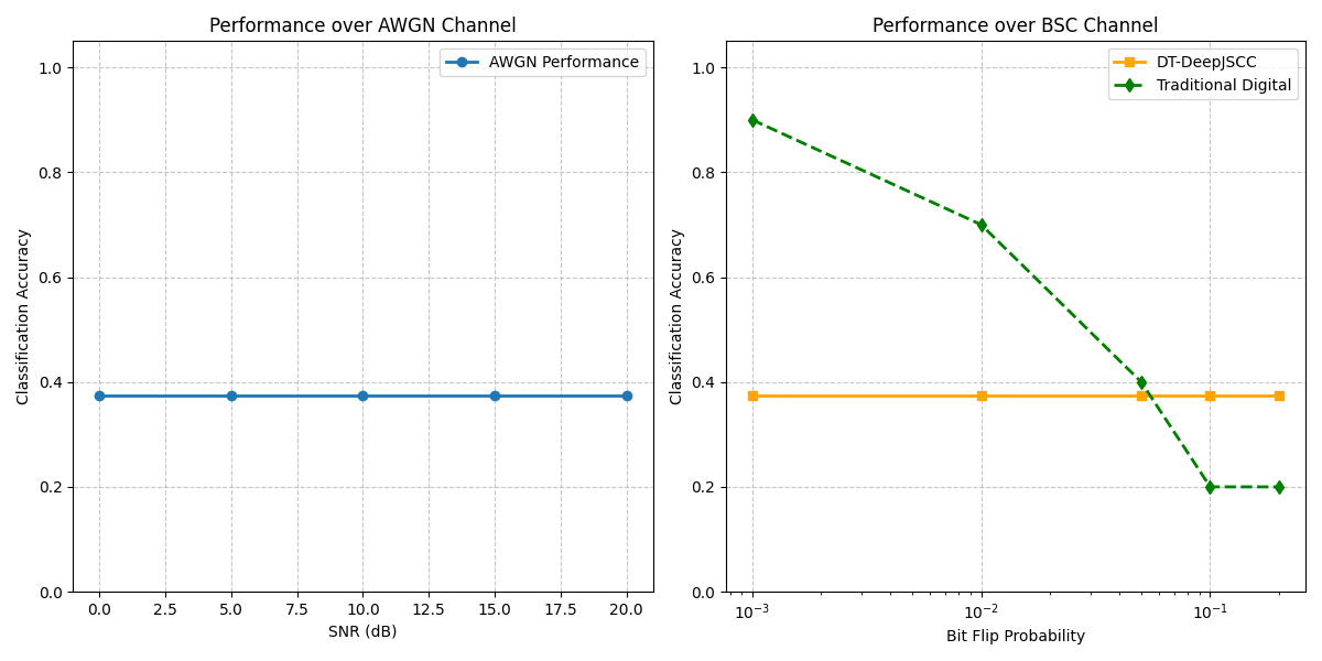
Total running time of the script: (0 minutes 3.535 seconds)
