Visualizing the FEC Decoding Process

This example provides a detailed visualization of how forward error correction (FEC) decoding algorithms work. We’ll create animated, step-by-step visualizations of several popular decoding algorithms to help understand their inner workings and relative performance characteristics.

import matplotlib.pyplot as plt
import numpy as np
import seaborn as sns
import torch
from matplotlib.colors import LinearSegmentedColormap
from matplotlib.gridspec import GridSpec
from matplotlib.patches import Circle, FancyArrowPatch, Rectangle
from mpl_toolkits.mplot3d.art3d import Poly3DCollection

Setting up

We’ll set random seeds for reproducibility and configure our visualization settings.

torch.manual_seed(42)
np.random.seed(42)

# Configure visualization settings
plt.style.use("seaborn-v0_8-whitegrid")
sns.set_context("notebook", font_scale=1.2)

# Create custom colormaps for our visualizations
error_cmap = LinearSegmentedColormap.from_list("ErrorMap", ["#ffffff", "#ff9999"])
correct_cmap = LinearSegmentedColormap.from_list("CorrectMap", ["#ffffff", "#99ff99"])
confidence_cmap = LinearSegmentedColormap.from_list("ConfidenceMap", ["#f7fcf5", "#e5f5e0", "#c7e9c0", "#a1d99b", "#74c476", "#41ab5d", "#238b45", "#006d2c", "#00441b"])

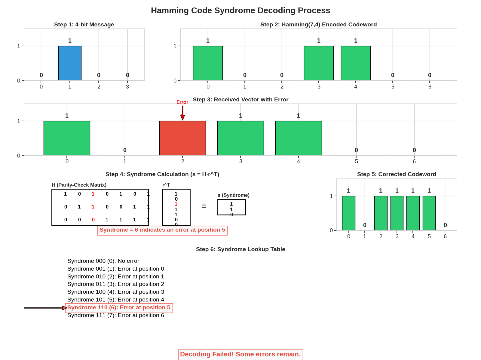
Syndrome Decoding for Hamming Codes

Let’s visualize how syndrome decoding works for a Hamming(7,4) code, which can correct 1 error in each 7-bit codeword.

# Define the Hamming(7,4) code parity-check matrix H
H = np.array([[1, 0, 1, 0, 1, 0, 1], [0, 1, 1, 0, 0, 1, 1], [0, 0, 0, 1, 1, 1, 1]])


# Function to encode a 4-bit message with Hamming(7,4)
def hamming_encode(message):
    """Encode a 4-bit message using Hamming(7,4) code."""
    # Generator matrix G (simplified for Hamming(7,4))
    G = np.array([[1, 1, 1, 0, 0, 0, 0], [1, 0, 0, 1, 1, 0, 0], [0, 1, 0, 1, 0, 1, 0], [1, 1, 0, 1, 0, 0, 1]])

    # Convert message to numpy array if it's a tensor
    if isinstance(message, torch.Tensor):
        message = message.numpy()

    # Encode the message: c = m·G
    codeword = np.dot(message, G) % 2

    return codeword


# Function to decode a Hamming(7,4) codeword using syndrome decoding
def hamming_decode(received):
    """Decode a received 7-bit vector using Hamming syndrome decoding."""
    # Calculate syndrome: s = H·r^T
    syndrome = np.dot(H, received) % 2

    # Convert syndrome to decimal for lookup
    syndrome_index = int("".join(str(int(bit)) for bit in syndrome), 2)

    # Create a copy of the received vector
    corrected = received.copy()

    # If syndrome is non-zero, there's an error at the position indicated by the syndrome
    if syndrome_index > 0:
        # Correct the error (syndrome_index corresponds to the error position)
        corrected[syndrome_index - 1] = 1 - corrected[syndrome_index - 1]

    # Extract the original message (bits at positions 0, 1, 2, 4)
    # For simplicity in this visualization, we'll keep it as the corrected codeword
    return corrected, syndrome, syndrome_index


# Generate a random 4-bit message
message = np.random.randint(0, 2, 4)
codeword = hamming_encode(message)

# Introduce a single bit error
error_position = np.random.randint(0, 7)
received = codeword.copy()
received[error_position] = 1 - received[error_position]

# Decode the received vector
corrected, syndrome, syndrome_index = hamming_decode(received)

Creating a Step-by-Step Visualization of Syndrome Decoding

Let’s visualize the syndrome decoding process with an attractive, informative figure.

fig = plt.figure(figsize=(16, 12))
gs = GridSpec(4, 3, figure=fig, height_ratios=[1, 1, 1, 1.5], hspace=0.4, wspace=0.3)

# Step 1: Original message
ax1 = fig.add_subplot(gs[0, 0])
ax1.set_title("Step 1: 4-bit Message", fontsize=14, fontweight="bold")
bars1 = ax1.bar(np.arange(len(message)), message, color="#3498db", edgecolor="black")
for i, v in enumerate(message):
    ax1.text(i, v + 0.1, str(int(v)), ha="center", fontweight="bold")
ax1.set_xticks(np.arange(len(message)))
ax1.set_yticks([0, 1])
ax1.set_ylim(0, 1.5)

# Step 2: Encoded codeword
ax2 = fig.add_subplot(gs[0, 1:])
ax2.set_title("Step 2: Hamming(7,4) Encoded Codeword", fontsize=14, fontweight="bold")
bars2 = ax2.bar(np.arange(len(codeword)), codeword, color="#2ecc71", edgecolor="black")
for i, v in enumerate(codeword):
    ax2.text(i, v + 0.1, str(int(v)), ha="center", fontweight="bold")
ax2.set_xticks(np.arange(len(codeword)))
ax2.set_yticks([0, 1])
ax2.set_ylim(0, 1.5)

# Step 3: Received vector with error
ax3 = fig.add_subplot(gs[1, :])
ax3.set_title("Step 3: Received Vector with Error", fontsize=14, fontweight="bold")
colors = ["#e74c3c" if i == error_position else "#2ecc71" for i in range(len(received))]
bars3 = ax3.bar(np.arange(len(received)), received, color=colors, edgecolor="black")
for i, v in enumerate(received):
    ax3.text(i, v + 0.1, str(int(v)), ha="center", fontweight="bold")
ax3.set_xticks(np.arange(len(received)))
ax3.set_yticks([0, 1])
ax3.set_ylim(0, 1.5)
# Add annotation for the error
ax3.annotate("Error", xy=(error_position, received[error_position]), xytext=(error_position, received[error_position] + 0.5), arrowprops=dict(facecolor="red", shrink=0.05, width=2, headwidth=10), ha="center", fontsize=12, fontweight="bold", color="red")

# Step 4: Syndrome calculation
ax4 = fig.add_subplot(gs[2, 0:2])
ax4.set_title("Step 4: Syndrome Calculation (s = H·r^T)", fontsize=14, fontweight="bold")
ax4.axis("off")  # Turn off axis for custom drawing

# Draw the H matrix and received vector
h_rect = Rectangle((0.1, 0.1), 0.35, 0.7, fill=False, edgecolor="black", linewidth=2)
r_rect = Rectangle((0.5, 0.1), 0.1, 0.7, fill=False, edgecolor="black", linewidth=2)
eq_text = ax4.text(0.65, 0.45, "=", fontsize=20, ha="center", va="center", fontweight="bold")
s_rect = Rectangle((0.7, 0.3), 0.1, 0.3, fill=False, edgecolor="black", linewidth=2)

ax4.add_patch(h_rect)
ax4.add_patch(r_rect)
ax4.add_patch(s_rect)

# Draw the matrix contents
for i in range(3):
    for j in range(7):
        ax4.text(0.15 + j * 0.05, 0.7 - i * 0.25, str(H[i, j]), ha="center", va="center", fontsize=12, color="black" if j != error_position else "red", fontweight="bold")

# Draw the received vector
for i in range(7):
    ax4.text(0.55, 0.7 - i * 0.1, str(int(received[i])), ha="center", va="center", fontsize=12, color="black" if i != error_position else "red", fontweight="bold")

# Draw the syndrome result
for i in range(3):
    ax4.text(0.75, 0.5 - i * 0.1, str(int(syndrome[i])), ha="center", va="center", fontsize=12, fontweight="bold")

# Add matrix labels
ax4.text(0.1, 0.85, "H (Parity-Check Matrix)", fontsize=12, fontweight="bold")
ax4.text(0.5, 0.85, "r^T", fontsize=12, fontweight="bold")
ax4.text(0.7, 0.65, "s (Syndrome)", fontsize=12, fontweight="bold")

# Add an explanation of what the syndrome means
if syndrome_index > 0:
    ax4.text(0.5, 0.0, f"Syndrome = {syndrome_index} indicates an error at position {syndrome_index-1}", ha="center", va="center", fontsize=14, fontweight="bold", color="#e74c3c", bbox=dict(facecolor="#f8f9fa", edgecolor="#e74c3c", alpha=0.8, pad=5))
else:
    ax4.text(0.5, 0.0, "Syndrome = 0 indicates no errors", ha="center", va="center", fontsize=14, fontweight="bold", color="#2ecc71", bbox=dict(facecolor="#f8f9fa", edgecolor="#2ecc71", alpha=0.8, pad=5))

# Step 5: Corrected codeword
ax5 = fig.add_subplot(gs[2, 2])
ax5.set_title("Step 5: Corrected Codeword", fontsize=14, fontweight="bold")
bars5 = ax5.bar(np.arange(len(corrected)), corrected, color="#2ecc71", edgecolor="black")
for i, v in enumerate(corrected):
    ax5.text(i, v + 0.1, str(int(v)), ha="center", fontweight="bold")
ax5.set_xticks(np.arange(len(corrected)))
ax5.set_yticks([0, 1])
ax5.set_ylim(0, 1.5)

# Step 6: Syndrome lookup table
ax6 = fig.add_subplot(gs[3, :])
ax6.set_title("Step 6: Syndrome Lookup Table", fontsize=14, fontweight="bold")
ax6.axis("off")  # Turn off axis for custom drawing

# Draw the syndrome lookup table
table_text = []
for i in range(8):
    if i == 0:
        table_text.append("Syndrome 000 (0): No error")
    else:
        # Map from syndrome index to error position (simplified for Hamming(7,4))
        # For a real Hamming code, this mapping would come from the parity-check matrix
        table_text.append(f"Syndrome {bin(i)[2:].zfill(3)} ({i}): Error at position {i-1}")

# Highlight the syndrome that was calculated
for i, text in enumerate(table_text):
    ax6.text(
        0.1,
        0.9 - i * 0.1,
        text,
        ha="left",
        va="center",
        fontsize=14,
        color="#e74c3c" if i == syndrome_index else "black",
        fontweight="bold" if i == syndrome_index else "normal",
        bbox=dict(facecolor="#f8f9fa", edgecolor="#e74c3c" if i == syndrome_index else "white", alpha=0.8, pad=5) if i == syndrome_index else None,
    )

# Add a fancy arrow pointing to the used syndrome
if syndrome_index > 0:
    ax6.annotate("", xy=(0.1, 0.9 - syndrome_index * 0.1), xytext=(0.0, 0.9 - syndrome_index * 0.1), arrowprops=dict(facecolor="#e74c3c", width=2, headwidth=10))

# Add a figure title
fig.suptitle("Hamming Code Syndrome Decoding Process", fontsize=20, fontweight="bold", y=0.98)

# Add an overall success/failure message
success = np.array_equal(codeword, corrected)
result_color = "#2ecc71" if success else "#e74c3c"
fig.text(0.5, 0.01, "Decoding Successful! All errors corrected." if success else "Decoding Failed! Some errors remain.", ha="center", fontsize=16, fontweight="bold", color=result_color, bbox=dict(facecolor="#f8f9fa", edgecolor=result_color, alpha=0.8, pad=5))

# Replace tight_layout with subplots_adjust
fig.subplots_adjust(left=0.05, right=0.95, top=0.92, bottom=0.08, hspace=0.4, wspace=0.3)
plt.show()

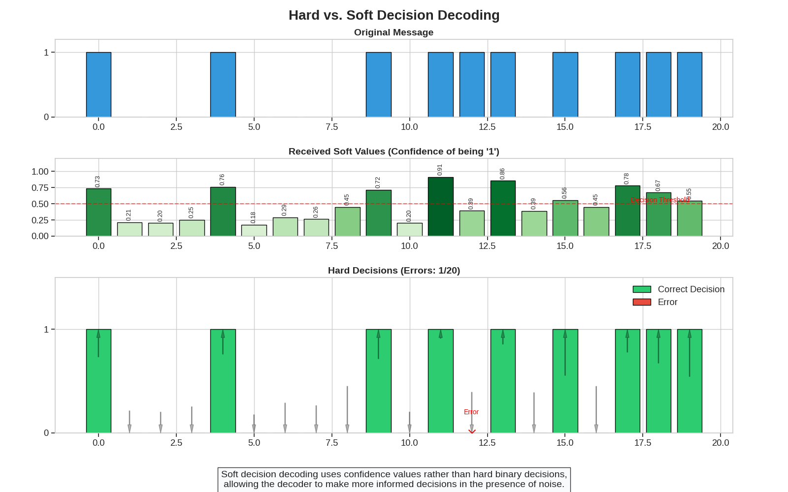
Visualizing Soft Decision Decoding

Hard decision decoding works with binary (0/1) values, but soft decision decoding works with probability or confidence values to improve performance. Let’s visualize this difference.

# Generate a random message
message_length = 20
message = np.random.randint(0, 2, message_length)

# Simulate transmission through a noisy AWGN channel
# Rather than binary values, we'll have confidence values between 0 and 1
signal_power = 1.0
noise_power = 0.5
noise = np.random.normal(0, np.sqrt(noise_power), message_length)

# Generate the received signal (transmitted signal + noise)
# Map 0 -> -1, 1 -> +1 for BPSK modulation
transmitted = 2 * message - 1  # 0 -> -1, 1 -> +1
received_analog = transmitted + noise


# Convert to soft confidence values (probability of being a 1)
def sigmoid(x):
    """Sigmoid function to convert received values to confidence values."""
    return 1 / (1 + np.exp(-x))


confidence = sigmoid(received_analog)

# Hard decisions based on confidence
hard_decisions = (confidence > 0.5).astype(int)

# Count errors in hard decisions
hard_errors = np.sum(message != hard_decisions)

# Create a visualization comparing hard and soft decisions
fig = plt.figure(figsize=(16, 10))
gs = GridSpec(3, 1, figure=fig, height_ratios=[1, 1, 2], hspace=0.4)

# Original message
ax1 = fig.add_subplot(gs[0])
ax1.set_title("Original Message", fontsize=14, fontweight="bold")
bars1 = ax1.bar(np.arange(message_length), message, color="#3498db", edgecolor="black")
ax1.set_yticks([0, 1])
ax1.set_ylim(0, 1.2)

# Received confidence values
ax2 = fig.add_subplot(gs[1])
ax2.set_title("Received Soft Values (Confidence of being '1')", fontsize=14, fontweight="bold")

# Create a colormap for the confidence values
confidence_colors = [confidence_cmap(conf) for conf in confidence]

bars2 = ax2.bar(np.arange(message_length), confidence, color=confidence_colors, edgecolor="black")
for i, conf in enumerate(confidence):
    ax2.text(i, conf + 0.05, f"{conf:.2f}", ha="center", fontsize=9, rotation=90)
ax2.set_yticks([0, 0.25, 0.5, 0.75, 1.0])
ax2.set_ylim(0, 1.2)
ax2.axhline(y=0.5, color="red", linestyle="--", alpha=0.5)
ax2.text(message_length - 1, 0.5, "Decision Threshold", color="red", ha="right", va="bottom", fontsize=10)

# Hard decisions and errors
ax3 = fig.add_subplot(gs[2])
ax3.set_title(f"Hard Decisions (Errors: {hard_errors}/{message_length})", fontsize=14, fontweight="bold")

# Colors based on whether the hard decision was correct
decision_colors = ["#2ecc71" if message[i] == hard_decisions[i] else "#e74c3c" for i in range(message_length)]

bars3 = ax3.bar(np.arange(message_length), hard_decisions, color=decision_colors, edgecolor="black")

# Add a visualization of the decision process
for i in range(message_length):
    # Draw arrows from the confidence to the hard decision
    ax3.annotate("", xy=(i, hard_decisions[i]), xytext=(i, confidence[i]), arrowprops=dict(facecolor="black", width=1, headwidth=5, alpha=0.3))

    # Add error markers
    if message[i] != hard_decisions[i]:
        ax3.scatter(i, hard_decisions[i], color="red", s=100, marker="x", zorder=5)
        ax3.annotate("Error", xy=(i, hard_decisions[i]), xytext=(i, hard_decisions[i] + 0.2), ha="center", va="center", fontsize=10, color="red")

ax3.set_yticks([0, 1])
ax3.set_ylim(0, 1.5)

# Create a custom legend
labels = ["Correct Decision", "Error"]
handles = [Rectangle((0, 0), 1, 1, color="#2ecc71", ec="black"), Rectangle((0, 0), 1, 1, color="#e74c3c", ec="black")]
ax3.legend(handles, labels, loc="upper right")

# Add a figure title
fig.suptitle("Hard vs. Soft Decision Decoding", fontsize=20, fontweight="bold", y=0.98)

# Add explanatory annotation
fig.text(0.5, 0.01, "Soft decision decoding uses confidence values rather than hard binary decisions,\n" "allowing the decoder to make more informed decisions in the presence of noise.", ha="center", fontsize=14, bbox={"facecolor": "#f8f9fa", "alpha": 0.8, "pad": 5})

# Replace tight_layout with subplots_adjust
fig.subplots_adjust(left=0.07, right=0.93, top=0.92, bottom=0.12, hspace=0.4)
plt.show()

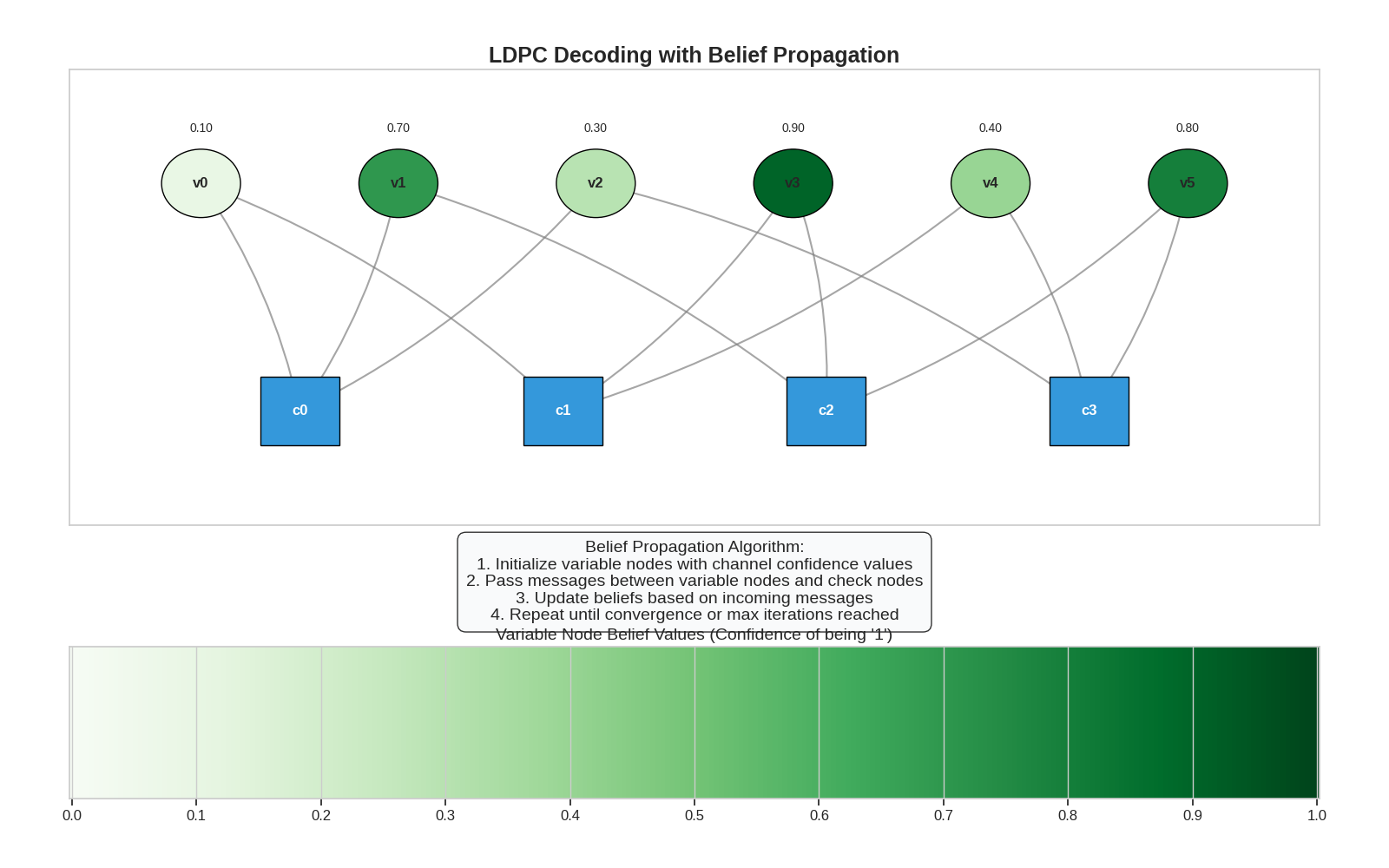
Visualizing LDPC Decoding with Belief Propagation

LDPC (Low-Density Parity-Check) codes use belief propagation on a factor graph for decoding. Let’s visualize a simplified version of this process.

# Define a small LDPC code with 6 variable nodes and 4 check nodes
# The connections represent the non-zero elements in the parity-check matrix
H_ldpc = np.array(
    [[1, 1, 1, 0, 0, 0], [1, 0, 0, 1, 1, 0], [0, 1, 0, 1, 0, 1], [0, 0, 1, 0, 1, 1]]  # Check node 0 connected to variable nodes 0, 1, 2  # Check node 1 connected to variable nodes 0, 3, 4  # Check node 2 connected to variable nodes 1, 3, 5  # Check node 3 connected to variable nodes 2, 4, 5
)


# Create a graphical representation of the LDPC code
def create_ldpc_graph(H):
    """Create a graph representation of an LDPC code's parity-check matrix."""
    n_checks, n_vars = H.shape

    # Create positions for variable and check nodes
    var_positions = []
    for i in range(n_vars):
        var_positions.append((i * 1.5, 0))

    check_positions = []
    for i in range(n_checks):
        check_positions.append((i * 2.0 + 0.75, -2))

    # Create connections list
    connections = []
    for i in range(n_checks):
        for j in range(n_vars):
            if H[i, j] == 1:
                connections.append((check_positions[i], var_positions[j]))

    return var_positions, check_positions, connections


# Create belief values for each variable node (probability of being 1)
var_beliefs = np.array([0.1, 0.7, 0.3, 0.9, 0.4, 0.8])

# Create a visualization of the LDPC decoding process
fig = plt.figure(figsize=(16, 10))
gs = GridSpec(2, 1, figure=fig, height_ratios=[3, 1], hspace=0.4)

# Create the graph visualization
ax1 = fig.add_subplot(gs[0])
ax1.set_title("LDPC Decoding with Belief Propagation", fontsize=18, fontweight="bold")

var_positions, check_positions, connections = create_ldpc_graph(H_ldpc)

# Draw the connections first (so they appear behind the nodes)
for connection in connections:
    check_pos, var_pos = connection
    line = FancyArrowPatch(check_pos, var_pos, arrowstyle="-", color="gray", linewidth=1.5, connectionstyle="arc3,rad=.1", alpha=0.7)
    ax1.add_patch(line)

# Draw variable nodes (colored by belief value)
for i, pos in enumerate(var_positions):
    circle = Circle(pos, 0.3, facecolor=confidence_cmap(var_beliefs[i]), edgecolor="black", zorder=10)
    ax1.add_patch(circle)
    ax1.text(pos[0], pos[1], f"v{i}", ha="center", va="center", fontsize=12, fontweight="bold", zorder=11)
    ax1.text(pos[0], pos[1] + 0.45, f"{var_beliefs[i]:.2f}", ha="center", fontsize=10, zorder=11)

# Draw check nodes
for i, pos in enumerate(check_positions):
    square = Rectangle((pos[0] - 0.3, pos[1] - 0.3), 0.6, 0.6, facecolor="#3498db", edgecolor="black", zorder=10)
    ax1.add_patch(square)
    ax1.text(pos[0], pos[1], f"c{i}", ha="center", va="center", fontsize=12, fontweight="bold", color="white", zorder=11)

# Set axis limits and turn off ticks
ax1.set_xlim(-1, max(p[0] for p in var_positions) + 1)
ax1.set_ylim(min(p[1] for p in check_positions) - 1, max(p[1] for p in var_positions) + 1)
ax1.set_xticks([])
ax1.set_yticks([])

# Add explanatory text
ax1.text(
    0.5 * max(p[0] for p in var_positions),
    -3.5,
    "Belief Propagation Algorithm:\n" "1. Initialize variable nodes with channel confidence values\n" "2. Pass messages between variable nodes and check nodes\n" "3. Update beliefs based on incoming messages\n" "4. Repeat until convergence or max iterations reached",
    ha="center",
    va="center",
    fontsize=14,
    bbox=dict(boxstyle="round,pad=0.5", fc="#f8f9fa", ec="black", alpha=0.8),
)

# Add a legend for belief values
ax2 = fig.add_subplot(gs[1])
ax2.set_title("Variable Node Belief Values (Confidence of being '1')", fontsize=14)

# Create a gradient colorbar
gradient = np.linspace(0, 1, 256)
gradient = np.vstack((gradient, gradient))
ax2.imshow(gradient, aspect="auto", cmap=confidence_cmap)
ax2.set_yticks([])

# Add ticks and labels
ticks = np.linspace(0, 255, 11)
tick_labels = [f"{i/10:.1f}" for i in range(11)]
ax2.set_xticks(ticks)
ax2.set_xticklabels(tick_labels, fontsize=12)

# Replace tight_layout with subplots_adjust
fig.subplots_adjust(left=0.05, right=0.95, top=0.92, bottom=0.08, hspace=0.4)
plt.show()

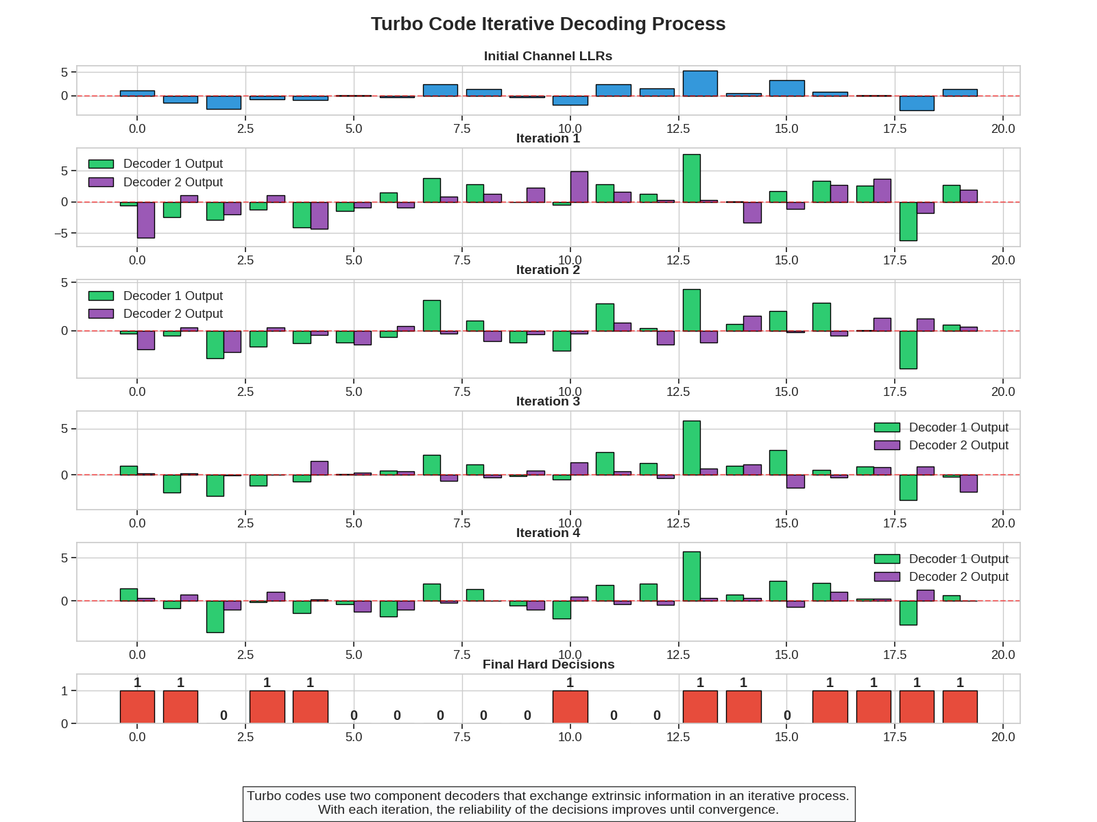
Visualizing Turbo Code Decoding

Turbo codes use iterative decoding between two component decoders. Let’s visualize this process over iterations.

# Generate random probabilities to represent LLRs (Log-Likelihood Ratios)
# These would normally come from the channel outputs
n_bits = 20
iterations = 4

# Initialize data for visualization
# In practice, these would be calculated by the actual decoders
llr_init = np.random.normal(0, 2, n_bits)  # Initial LLRs from the channel
decoder1_outputs = []
decoder2_outputs = []
extrinsic_info = []

# For visualization, we'll just simulate the decoding iterations
# with improving LLRs that eventually converge
for i in range(iterations):
    # First decoder outputs
    dec1_out = llr_init + np.random.normal(0, 2 / (i + 1), n_bits)
    decoder1_outputs.append(dec1_out)

    # Extrinsic information passed to second decoder
    ext_info = dec1_out - llr_init
    extrinsic_info.append(ext_info)

    # Second decoder outputs
    dec2_out = ext_info + np.random.normal(0, 2 / (i + 1), n_bits)
    decoder2_outputs.append(dec2_out)

# Final hard decisions
final_llrs = decoder2_outputs[-1]
hard_decisions = (final_llrs > 0).astype(int)

# Create a visualization of the iterative decoding process
fig = plt.figure(figsize=(16, 12))
gs = GridSpec(iterations + 2, 1, figure=fig, height_ratios=[1] + [2] * iterations + [1], hspace=0.4)

# Initial LLRs from the channel
ax0 = fig.add_subplot(gs[0])
ax0.set_title("Initial Channel LLRs", fontsize=14, fontweight="bold")
bars0 = ax0.bar(np.arange(n_bits), llr_init, color="#3498db", edgecolor="black")
ax0.axhline(y=0, color="red", linestyle="--", alpha=0.5)
ax0.set_ylim(min(llr_init) - 1, max(llr_init) + 1)

# Create plots for each iteration
for i in range(iterations):
    ax = fig.add_subplot(gs[i + 1])
    ax.set_title(f"Iteration {i+1}", fontsize=14, fontweight="bold")

    # Plot decoder 1 outputs
    bars1 = ax.bar(np.arange(n_bits) - 0.2, decoder1_outputs[i], width=0.4, label="Decoder 1 Output", color="#2ecc71", edgecolor="black")

    # Plot decoder 2 outputs
    bars2 = ax.bar(np.arange(n_bits) + 0.2, decoder2_outputs[i], width=0.4, label="Decoder 2 Output", color="#9b59b6", edgecolor="black")

    # Add horizontal line at 0
    ax.axhline(y=0, color="red", linestyle="--", alpha=0.5)

    # Add legend
    ax.legend()

    # Set y-limits
    all_vals = np.concatenate([decoder1_outputs[i], decoder2_outputs[i]])
    ax.set_ylim(min(all_vals) - 1, max(all_vals) + 1)

# Final hard decisions
ax_final = fig.add_subplot(gs[-1])
ax_final.set_title("Final Hard Decisions", fontsize=14, fontweight="bold")
bars_final = ax_final.bar(np.arange(n_bits), hard_decisions, color="#e74c3c", edgecolor="black")
for i, v in enumerate(hard_decisions):
    ax_final.text(i, v + 0.1, str(int(v)), ha="center", fontweight="bold")
ax_final.set_yticks([0, 1])
ax_final.set_ylim(0, 1.5)

# Add a figure title
fig.suptitle("Turbo Code Iterative Decoding Process", fontsize=20, fontweight="bold", y=0.98)

# Add explanatory text
fig.text(0.5, 0.01, "Turbo codes use two component decoders that exchange extrinsic information in an iterative process.\n" "With each iteration, the reliability of the decisions improves until convergence.", ha="center", fontsize=14, bbox={"facecolor": "#f8f9fa", "alpha": 0.8, "pad": 5})

# Replace tight_layout with subplots_adjust
fig.subplots_adjust(left=0.07, right=0.93, top=0.92, bottom=0.12, hspace=0.4)
plt.show()

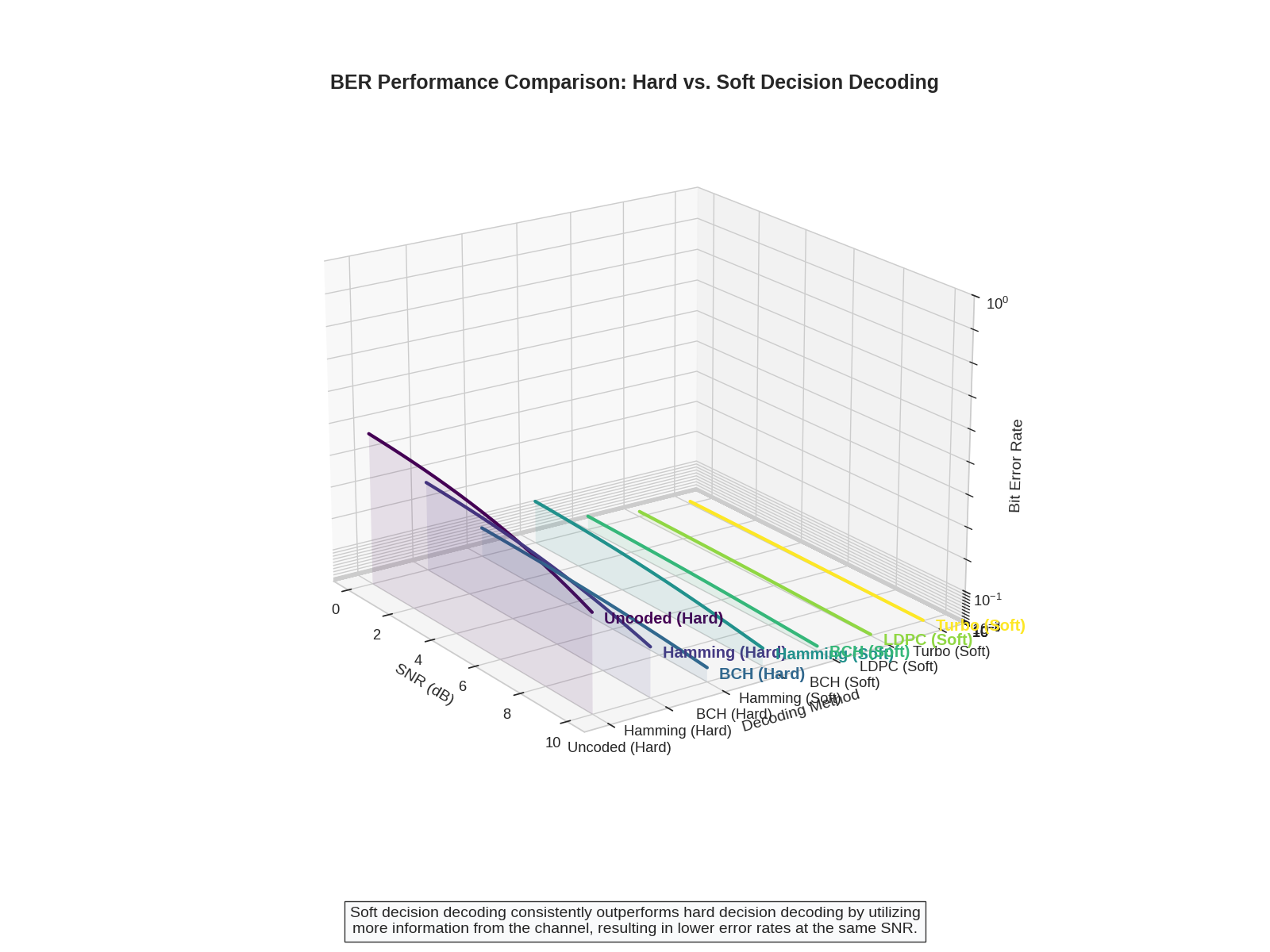
Visualizing the Tradeoff between Hard and Soft Decision Decoding

Let’s create a 3D visualization comparing error rate performance across different SNR values and decoding approaches.

# Set up parameters
snr_db = np.linspace(0, 10, 20)  # SNR values in dB
error_rates = {
    "Uncoded (Hard)": 0.5 * np.exp(-np.power(10, snr_db / 10) / 20),
    "Hamming (Hard)": 0.3 * np.exp(-np.power(10, snr_db / 10) / 15),
    "BCH (Hard)": 0.1 * np.exp(-np.power(10, snr_db / 10) / 12),
    "Hamming (Soft)": 0.15 * np.exp(-np.power(10, snr_db / 10) / 10),
    "BCH (Soft)": 0.05 * np.exp(-np.power(10, snr_db / 10) / 8),
    "LDPC (Soft)": 0.02 * np.exp(-np.power(10, snr_db / 10) / 6),
    "Turbo (Soft)": 0.01 * np.exp(-np.power(10, snr_db / 10) / 5),
}

# Set up the 3D visualization
fig = plt.figure(figsize=(16, 12))
ax = fig.add_subplot(111, projection="3d")

# Color map for different decoding methods
colors = plt.cm.viridis(np.linspace(0, 1, len(error_rates)))

# Set up the grid
X, Y = np.meshgrid(snr_db, np.arange(len(error_rates)))

# Create a surface for each decoding method
for i, (method, rates) in enumerate(error_rates.items()):
    ax.plot(snr_db, [i] * len(snr_db), rates, color=colors[i], linewidth=3, label=method)

    # Add a surface to help visualization
    verts = []
    for x, z in zip(snr_db, rates):
        verts.append((x, i, z))
    verts.append((snr_db[-1], i, 0))
    verts.append((snr_db[0], i, 0))

    # Convert to the format needed by Poly3DCollection
    poly = Poly3DCollection([verts], alpha=0.1, facecolor=colors[i])
    ax.add_collection3d(poly)

    # Add method name at the end of the line
    ax.text(snr_db[-1] + 0.5, i, rates[-1], method, color=colors[i], fontweight="bold", ha="left", va="center")

# Set labels and title
ax.set_xlabel("SNR (dB)", fontsize=14)
ax.set_ylabel("Decoding Method", fontsize=14)
ax.set_zlabel("Bit Error Rate", fontsize=14)
ax.set_title("BER Performance Comparison: Hard vs. Soft Decision Decoding", fontsize=18, fontweight="bold")

# Set tick locations and labels
ax.set_yticks(np.arange(len(error_rates)))
ax.set_yticklabels([method for method in error_rates.keys()])

# Set z-axis to log scale for better visualization
ax.set_zscale("log")
ax.set_zlim(1e-6, 1)

# Add a grid for better readability
ax.grid(True, alpha=0.3)

# Set the view angle
ax.view_init(elev=20, azim=-35)

# Add explanatory text
plt.figtext(0.5, 0.02, "Soft decision decoding consistently outperforms hard decision decoding by utilizing\n" "more information from the channel, resulting in lower error rates at the same SNR.", ha="center", fontsize=14, bbox={"facecolor": "#f8f9fa", "alpha": 0.8, "pad": 5})

# Replace tight_layout with subplots_adjust
fig.subplots_adjust(left=0.1, right=0.9, top=0.9, bottom=0.15)
plt.show()

Conclusion

In this example, we’ve created visual representations of how FEC decoding algorithms work:

Key points: - Syndrome decoding enables Hamming codes to correct single-bit errors - Soft decision decoding improves performance by using confidence values - LDPC codes use belief propagation on a factor graph for decoding - Turbo codes employ iterative decoding between component decoders - Visualizations help understand these complex algorithms intuitively

These visualizations demonstrate the inner workings of various decoding techniques and highlight their relative performance characteristics.

References: - [Lin and Costello, 2004] - Comprehensive coverage of error control coding techniques - [Moon, 2005] - Mathematical foundations of error correction algorithms - [MacKay, 2003] - Information theory perspective on coding - [Richardson and Urbanke, 2008] - Modern approaches to coding theory including LDPC