Practical Applications of Constraints in Wireless Communication Systems

This example demonstrates practical applications of Kaira’s constraints in realistic wireless communication scenarios, focusing on OFDM and MIMO systems. We’ll explore how to configure and apply appropriate constraints for these systems.

Imports and Setup

We start by importing the necessary modules and setting up the environment.

import matplotlib.pyplot as plt
import numpy as np
import torch
from matplotlib.gridspec import GridSpec

from kaira.constraints import PAPRConstraint, PeakAmplitudeConstraint, TotalPowerConstraint
from kaira.constraints.utils import (
    apply_constraint_chain,
    combine_constraints,
    create_mimo_constraints,
    create_ofdm_constraints,
    measure_signal_properties,
    verify_constraint,
)

# Set random seed for reproducibility
torch.manual_seed(42)
np.random.seed(42)

Part 1: OFDM System Constraints

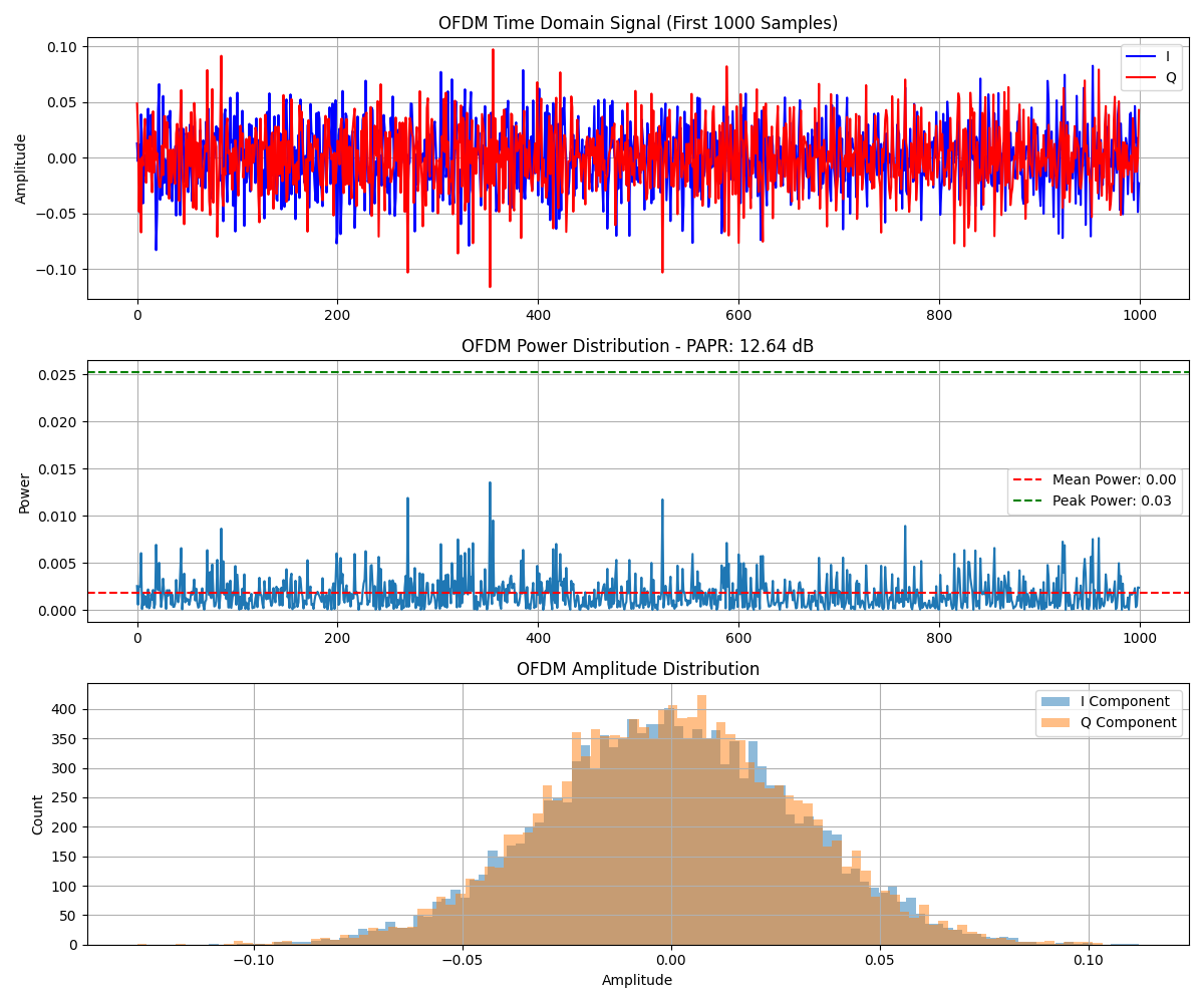
OFDM (Orthogonal Frequency Division Multiplexing) is widely used in modern communication systems like Wi-Fi, 5G, and digital broadcasting. OFDM signals typically require constraints to control their high PAPR (Peak-to-Average Power Ratio).

# Create an OFDM signal (simplified)
n_subcarriers = 1024
n_symbols = 10
CP_length = n_subcarriers // 4  # Cyclic prefix length

# Create random frequency-domain OFDM symbols
X_freq = torch.complex(torch.randn(1, n_symbols, n_subcarriers), torch.randn(1, n_symbols, n_subcarriers))

# Zero out DC and edge subcarriers (as in real OFDM systems)
X_freq[:, :, 0] = 0  # DC
guard_band = int(0.05 * n_subcarriers)  # 5% guard band on each edge
X_freq[:, :, -guard_band:] = 0
X_freq[:, :, :guard_band] = 0

# Convert to time domain with IFFT
X_time = torch.fft.ifft(X_freq, dim=2)

# Add cyclic prefix
cp_indices = torch.arange(n_subcarriers - CP_length, n_subcarriers)
with_cp = []
for i in range(n_symbols):
    symbol = X_time[:, i, :]
    cp = symbol[:, cp_indices]
    with_cp.append(torch.cat([cp, symbol], dim=1))

# Create final OFDM signal
ofdm_signal = torch.cat(with_cp, dim=1)

# Convert to real representation (I/Q components)
ofdm_iq = torch.cat([ofdm_signal.real, ofdm_signal.imag], dim=0)

# Display properties of the original OFDM signal
ofdm_props = measure_signal_properties(ofdm_iq)
print("Original OFDM Signal Properties:")
print(f"  Shape: {ofdm_iq.shape} (2 components, {ofdm_iq.shape[1]} samples)")
print(f"  Power: {ofdm_props['mean_power']:.4f}")
print(f"  PAPR: {ofdm_props['papr']:.2f} ({ofdm_props['papr_db']:.2f} dB)")
print(f"  Peak Amplitude: {ofdm_props['peak_amplitude']:.4f}")

Original OFDM Signal Properties:
  Shape: torch.Size([2, 12800]) (2 components, 12800 samples)
  Power: 0.0009
  PAPR: 18.36 (12.64 dB)
  Peak Amplitude: 0.1279

OFDM Signal Analysis

First, let’s analyze the original OFDM signal characteristics.

# Calculate time and frequency vectors for plotting
t = np.arange(ofdm_iq.shape[1])
signal_i = ofdm_iq[0].numpy()
signal_q = ofdm_iq[1].numpy()

# Plot time domain representation of original OFDM signal
plt.figure(figsize=(12, 10))

plt.subplot(3, 1, 1)
plt.plot(t[:1000], signal_i[:1000], "b-", label="I")
plt.plot(t[:1000], signal_q[:1000], "r-", label="Q")
plt.title("OFDM Time Domain Signal (First 1000 Samples)")
plt.grid(True)
plt.ylabel("Amplitude")
plt.legend()

# Compute and plot power distribution
power = signal_i**2 + signal_q**2
plt.subplot(3, 1, 2)
plt.plot(t[:1000], power[:1000])
plt.axhline(y=np.mean(power), color="r", linestyle="--", label=f"Mean Power: {np.mean(power):.2f}")
plt.axhline(y=np.max(power), color="g", linestyle="--", label=f"Peak Power: {np.max(power):.2f}")
plt.title(f"OFDM Power Distribution - PAPR: {ofdm_props['papr_db']:.2f} dB")
plt.grid(True)
plt.ylabel("Power")
plt.legend()

# Plot histogram of amplitudes
plt.subplot(3, 1, 3)
plt.hist(signal_i, bins=100, alpha=0.5, label="I Component")
plt.hist(signal_q, bins=100, alpha=0.5, label="Q Component")
plt.title("OFDM Amplitude Distribution")
plt.grid(True)
plt.xlabel("Amplitude")
plt.ylabel("Count")
plt.legend()

plt.tight_layout()
plt.show()

Applying OFDM Constraints

Let’s configure and apply appropriate constraints for the OFDM signal.

# Create OFDM constraints using the factory function
ofdm_constraints = create_ofdm_constraints(total_power=1.0, max_papr=6.0, is_complex=True, peak_amplitude=2.5)  # Normalize total power to 1.0  # Limit PAPR to 6 (approximately 7.8 dB)  # Signal has I/Q components  # Limit maximum amplitude

# Apply constraints to the OFDM signal
constrained_ofdm = ofdm_constraints(ofdm_iq.clone())

# Measure properties of the constrained signal
constrained_props = measure_signal_properties(constrained_ofdm)
print("\nConstrained OFDM Signal Properties:")
print(f"  Power: {constrained_props['mean_power']:.4f}")
print(f"  PAPR: {constrained_props['papr']:.2f} ({constrained_props['papr_db']:.2f} dB)")
print(f"  Peak Amplitude: {constrained_props['peak_amplitude']:.4f}")

# Alternative approach: apply individual constraints sequentially with verbose output
print("\nSequential Application of OFDM Constraints:")
constraints_list = [TotalPowerConstraint(total_power=1.0), PAPRConstraint(max_papr=6.0), PeakAmplitudeConstraint(max_amplitude=2.5)]

sequential_ofdm = apply_constraint_chain(constraints_list, ofdm_iq.clone())
sequential_props = measure_signal_properties(sequential_ofdm)

Constrained OFDM Signal Properties:
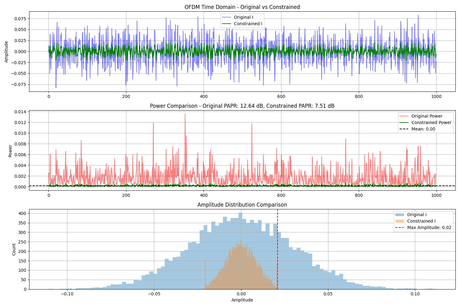
  Power: 0.0001
  PAPR: 5.64 (7.51 dB)
  Peak Amplitude: 0.0210

Sequential Application of OFDM Constraints:

Visualizing OFDM Constraint Effects

# Extract I/Q components for visualization
constrained_i = constrained_ofdm[0].numpy()
constrained_q = constrained_ofdm[1].numpy()
constrained_power = constrained_i**2 + constrained_q**2

# Compare original vs constrained signals
plt.figure(figsize=(15, 10))

# Time domain comparison
plt.subplot(3, 1, 1)
plt.plot(t[:1000], signal_i[:1000], "b-", alpha=0.5, label="Original I")
plt.plot(t[:1000], constrained_i[:1000], "g-", label="Constrained I")
plt.title("OFDM Time Domain - Original vs Constrained")
plt.grid(True)
plt.ylabel("Amplitude")
plt.legend()

# Power comparison
plt.subplot(3, 1, 2)
plt.plot(t[:1000], power[:1000], "r-", alpha=0.5, label="Original Power")
plt.plot(t[:1000], constrained_power[:1000], "g-", label="Constrained Power")
plt.axhline(y=np.mean(constrained_power), color="k", linestyle="--", label=f"Mean: {np.mean(constrained_power):.2f}")
plt.title(f"Power Comparison - Original PAPR: {ofdm_props['papr_db']:.2f} dB, " f"Constrained PAPR: {constrained_props['papr_db']:.2f} dB")
plt.grid(True)
plt.ylabel("Power")
plt.legend()

# Amplitude distribution comparison
plt.subplot(3, 1, 3)
plt.hist(signal_i, bins=100, alpha=0.4, label="Original I")
plt.hist(constrained_i, bins=100, alpha=0.4, label="Constrained I")
plt.axvline(x=constrained_props["peak_amplitude"], color="r", linestyle="--", label=f'Max Amplitude: {constrained_props["peak_amplitude"]:.2f}')
plt.title("Amplitude Distribution Comparison")
plt.grid(True)
plt.xlabel("Amplitude")
plt.ylabel("Count")
plt.legend()

plt.tight_layout()
plt.show()

Verify OFDM Constraint Effectiveness

Let’s verify that our constraints achieved their goals

# Verify power constraint
power_result = verify_constraint(TotalPowerConstraint(total_power=1.0), ofdm_iq.clone(), "power", 1.0, tolerance=1e-4)
print(f"Power constraint verification: {power_result}")

# Verify PAPR constraint
papr_result = verify_constraint(PAPRConstraint(max_papr=6.0), sequential_ofdm.clone(), "papr", 6.0, tolerance=1e-3)  # Use output from sequential application
print(f"PAPR constraint verification: {papr_result}")

# Verify amplitude constraint
amplitude_result = verify_constraint(PeakAmplitudeConstraint(max_amplitude=2.5), constrained_ofdm.clone(), "amplitude", 2.5, tolerance=1e-4)
print(f"Amplitude constraint verification: {amplitude_result}")

Power constraint verification: {'input_shape': torch.Size([2, 12800]), 'output_shape': torch.Size([2, 12800]), 'success': False, 'measured_power': 2.0, 'expected_power': 1.0}
PAPR constraint verification: {'input_shape': torch.Size([2, 12800]), 'output_shape': torch.Size([2, 12800]), 'success': True, 'measured_papr': 5.613608117469202, 'expected_papr': 6.0}
Amplitude constraint verification: {'input_shape': torch.Size([2, 12800]), 'output_shape': torch.Size([2, 12800]), 'success': True, 'measured_max_amplitude': 0.020982006564736366, 'expected_max_amplitude': 2.5}

Part 2: MIMO System Constraints

MIMO (Multiple-Input Multiple-Output) systems use multiple antennas to improve communication performance. Each antenna typically has its own power constraints.

# Define MIMO system parameters
n_antennas = 4
n_symbols = 50
n_subcarriers = 64

# Create a random MIMO signal
mimo_signal = torch.complex(torch.randn(n_antennas, n_symbols * n_subcarriers), torch.randn(n_antennas, n_symbols * n_subcarriers))

# Display properties of the original MIMO signal
print("\nOriginal MIMO Signal Properties:")
print(f"  Shape: {mimo_signal.shape} ({n_antennas} antennas, {mimo_signal.shape[1]} samples per antenna)")

# Calculate per-antenna power
per_antenna_power = []
for i in range(n_antennas):
    antenna_power = torch.mean(torch.abs(mimo_signal[i]) ** 2).item()
    per_antenna_power.append(antenna_power)
    print(f"  Antenna {i+1} Power: {antenna_power:.4f}")

print(f"  Total Power: {sum(per_antenna_power):.4f}")

Original MIMO Signal Properties:
  Shape: torch.Size([4, 3200]) (4 antennas, 3200 samples per antenna)
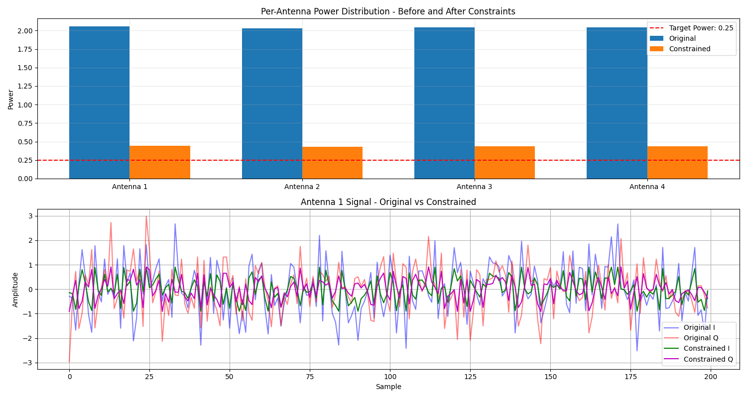
  Antenna 1 Power: 2.0583
  Antenna 2 Power: 2.0300
  Antenna 3 Power: 2.0446
  Antenna 4 Power: 2.0424
  Total Power: 8.1753

Applying MIMO Constraints

Let’s configure and apply appropriate constraints for the MIMO system.

# Create MIMO constraints using the factory function
# Set uniform power distribution across antennas
uniform_power = 0.25  # Total power 1.0 divided by 4 antennas
mimo_constraints = create_mimo_constraints(num_antennas=n_antennas, uniform_power=uniform_power, max_papr=4.0)  # Limit PAPR to 4 (approximately 6 dB)

# Apply constraints to the MIMO signal (convert to real first)
mimo_real = torch.cat([mimo_signal.real, mimo_signal.imag], dim=0)
constrained_mimo = mimo_constraints(mimo_real.clone())

# Reshape back to separate antennas and I/Q components
n_total = constrained_mimo.shape[0]
constrained_mimo_i = constrained_mimo[: n_total // 2]
constrained_mimo_q = constrained_mimo[n_total // 2 :]

# Calculate per-antenna power after constraints
print("\nConstrained MIMO Signal Properties:")
per_antenna_power_constrained = []
for i in range(n_antennas):
    antenna_power_i = torch.mean(constrained_mimo_i[i] ** 2).item()
    antenna_power_q = torch.mean(constrained_mimo_q[i] ** 2).item()
    antenna_power = antenna_power_i + antenna_power_q
    per_antenna_power_constrained.append(antenna_power)
    print(f"  Antenna {i+1} Power: {antenna_power:.4f}")

print(f"  Total Power: {sum(per_antenna_power_constrained):.4f}")

Constrained MIMO Signal Properties:
  Antenna 1 Power: 0.4449
  Antenna 2 Power: 0.4332
  Antenna 3 Power: 0.4381
  Antenna 4 Power: 0.4375
  Total Power: 1.7537

Visualizing MIMO Constraint Effects

# Plot original vs constrained power for each antenna
plt.figure(figsize=(15, 8))

# Power distribution
x_labels = [f"Antenna {i+1}" for i in range(n_antennas)]
x_pos = np.arange(len(x_labels))
width = 0.35

plt.subplot(2, 1, 1)
plt.bar(x_pos - width / 2, per_antenna_power, width, label="Original")
plt.bar(x_pos + width / 2, per_antenna_power_constrained, width, label="Constrained")
plt.axhline(y=uniform_power, color="r", linestyle="--", label=f"Target Power: {uniform_power:.2f}")
plt.ylabel("Power")
plt.title("Per-Antenna Power Distribution - Before and After Constraints")
plt.xticks(x_pos, x_labels)
plt.legend()
plt.grid(True, alpha=0.3)

# Time domain signal for one antenna
antenna_idx = 0
plt.subplot(2, 1, 2)
plt.plot(mimo_signal[antenna_idx].real.numpy()[:200], "b-", alpha=0.5, label="Original I")
plt.plot(mimo_signal[antenna_idx].imag.numpy()[:200], "r-", alpha=0.5, label="Original Q")
plt.plot(constrained_mimo_i[antenna_idx].numpy()[:200], "g-", label="Constrained I")
plt.plot(constrained_mimo_q[antenna_idx].numpy()[:200], "m-", label="Constrained Q")
plt.title(f"Antenna {antenna_idx+1} Signal - Original vs Constrained")
plt.grid(True)
plt.xlabel("Sample")
plt.ylabel("Amplitude")
plt.legend()

plt.tight_layout()
plt.show()

Adding Spectral Constraints to MIMO

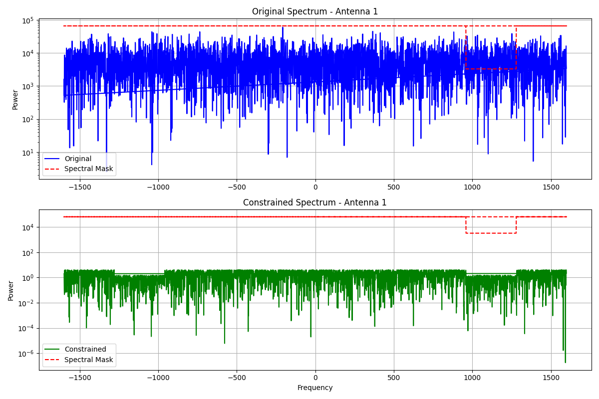
Let’s add spectral mask constraints to our MIMO system to simulate regulatory requirements.

# Create a spectral mask (e.g., simulating regulatory band restrictions)
spectral_mask = torch.ones(n_symbols * n_subcarriers)
# Create a restricted band
restricted_start = int(0.3 * n_symbols * n_subcarriers)
restricted_end = int(0.4 * n_symbols * n_subcarriers)
spectral_mask[restricted_start:restricted_end] = 0.05  # Severe attenuation

# Add spectral mask constraint to our MIMO constraint set
advanced_mimo_constraints = create_mimo_constraints(num_antennas=n_antennas, uniform_power=uniform_power, max_papr=4.0, spectral_mask=spectral_mask)

# Apply advanced constraints
advanced_constrained_mimo = advanced_mimo_constraints(mimo_real.clone())

# Calculate frequency spectra for visualization
antenna_idx = 0  # Choose one antenna for visualization
original_i = mimo_signal[antenna_idx].real.numpy()
original_q = mimo_signal[antenna_idx].imag.numpy()
original_spectrum = np.abs(np.fft.fft(original_i + 1j * original_q)) ** 2

advanced_i = advanced_constrained_mimo[antenna_idx].numpy()
advanced_q = advanced_constrained_mimo[n_antennas + antenna_idx].numpy()
advanced_spectrum = np.abs(np.fft.fft(advanced_i + 1j * advanced_q)) ** 2

# Visualize spectral constraints
plt.figure(figsize=(12, 8))
freq = np.fft.fftfreq(len(original_spectrum)) * len(original_spectrum)
mask_for_plot = spectral_mask.numpy() * np.max(original_spectrum) * 1.1

plt.subplot(2, 1, 1)
plt.semilogy(freq, original_spectrum, "b-", label="Original")
plt.semilogy(freq, mask_for_plot, "r--", label="Spectral Mask")
plt.title(f"Original Spectrum - Antenna {antenna_idx+1}")
plt.grid(True)
plt.ylabel("Power")
plt.legend()

plt.subplot(2, 1, 2)
plt.semilogy(freq, advanced_spectrum, "g-", label="Constrained")
plt.semilogy(freq, mask_for_plot, "r--", label="Spectral Mask")
plt.title(f"Constrained Spectrum - Antenna {antenna_idx+1}")
plt.grid(True)
plt.xlabel("Frequency")
plt.ylabel("Power")
plt.legend()

plt.tight_layout()
plt.show()

Part 3: Real-world Application - Complete OFDM Transmitter Constraints

Let’s put everything together to simulate a complete OFDM transmitter with practical constraints.

# Create a more complex OFDM signal with pilot symbols and data
n_sc = 256
n_sym = 20
cp_len = 32
pilot_interval = 4  # Insert pilot every 4 subcarriers

# Create subcarrier mapping
subcarrier_map = torch.zeros(n_sym, n_sc, dtype=torch.complex64)
data_indices = torch.ones(n_sc, dtype=bool)

# Add pilots at regular intervals
pilot_indices = torch.arange(0, n_sc, pilot_interval)
data_indices[pilot_indices] = False
pilots = torch.complex(torch.ones(pilot_indices.shape), torch.zeros(pilot_indices.shape))

# Add guard bands (null subcarriers)
guard_ratio = 0.1
guard_size = int(n_sc * guard_ratio)
data_indices[:guard_size] = False
data_indices[-guard_size:] = False

# Add DC null
dc_idx = n_sc // 2
data_indices[dc_idx] = False

# Map data and pilots
for i in range(n_sym):
    # Place pilots
    subcarrier_map[i, pilot_indices] = pilots

    # Place random QPSK data on data subcarriers
    n_data = torch.sum(data_indices).item()
    qpsk_real = torch.randint(0, 2, (n_data,)) * 2 - 1
    qpsk_imag = torch.randint(0, 2, (n_data,)) * 2 - 1
    qpsk_data = torch.complex(qpsk_real.float(), qpsk_imag.float())

    subcarrier_map[i, data_indices] = qpsk_data

# Convert to time domain signal
tx_ofdm = torch.fft.ifft(subcarrier_map, dim=1)

# Add cyclic prefix
tx_with_cp = []
for i in range(n_sym):
    symbol = tx_ofdm[i, :]
    cp = symbol[-cp_len:]
    tx_with_cp.append(torch.cat([cp, symbol]))

# Create final OFDM signal
ofdm_full = torch.cat(tx_with_cp)

# Convert to I/Q components for constraints
ofdm_iq_full = torch.stack([ofdm_full.real, ofdm_full.imag], dim=0)

# Measure original signal properties
ofdm_full_props = measure_signal_properties(ofdm_iq_full)
print("\nComplete OFDM Transmitter Signal Properties:")
print(f"  Shape: {ofdm_iq_full.shape}")
print(f"  Power: {ofdm_full_props['mean_power']:.4f}")
print(f"  PAPR: {ofdm_full_props['papr']:.2f} ({ofdm_full_props['papr_db']:.2f} dB)")
print(f"  Peak Amplitude: {ofdm_full_props['peak_amplitude']:.4f}")

Complete OFDM Transmitter Signal Properties:
  Shape: torch.Size([2, 5760])
  Power: 0.0028
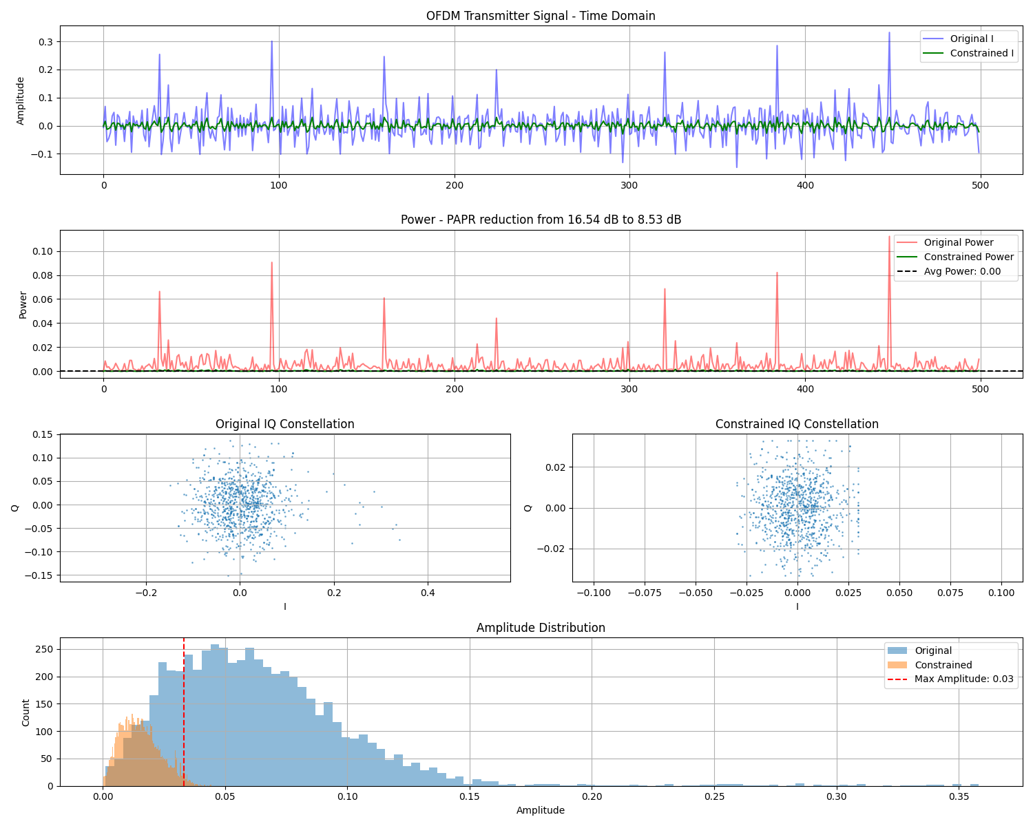
  PAPR: 45.06 (16.54 dB)
  Peak Amplitude: 0.3555

Applying Transmitter Constraints

Apply practical constraints for a realistic OFDM transmitter.

# Create combined transmitter constraints
tx_constraints = combine_constraints(
    [
        # Normalize total power
        TotalPowerConstraint(total_power=1.0),
        # Limit PAPR to realistic PA value
        PAPRConstraint(max_papr=7.0),  # ~8.5 dB
        # Limit peak amplitude for D/A converter
        PeakAmplitudeConstraint(max_amplitude=2.0),
    ]
)

# Apply constraints
tx_constrained = tx_constraints(ofdm_iq_full.clone())
tx_constrained_props = measure_signal_properties(tx_constrained)

print("\nConstrained Transmitter Signal Properties:")
print(f"  Power: {tx_constrained_props['mean_power']:.4f}")
print(f"  PAPR: {tx_constrained_props['papr']:.2f} ({tx_constrained_props['papr_db']:.2f} dB)")
print(f"  Peak Amplitude: {tx_constrained_props['peak_amplitude']:.4f}")

Constrained Transmitter Signal Properties:
  Power: 0.0002
  PAPR: 7.13 (8.53 dB)
  Peak Amplitude: 0.0331

Final Visualization and Analysis

Let’s visualize and analyze our transmitter signal before and after constraints.

# Time domain comparison
fig = plt.figure(figsize=(15, 12))
gs = GridSpec(4, 2, figure=fig)

# Plot time domain signals
t_segment = slice(0, 500)
plt.subplot(gs[0, :])
plt.plot(ofdm_iq_full[0, t_segment].numpy(), "b-", alpha=0.5, label="Original I")
plt.plot(tx_constrained[0, t_segment].numpy(), "g-", label="Constrained I")
plt.title("OFDM Transmitter Signal - Time Domain")
plt.grid(True)
plt.ylabel("Amplitude")
plt.legend()

# Plot power
orig_power = ofdm_iq_full[0].numpy() ** 2 + ofdm_iq_full[1].numpy() ** 2
const_power = tx_constrained[0].numpy() ** 2 + tx_constrained[1].numpy() ** 2

plt.subplot(gs[1, :])
plt.plot(orig_power[t_segment], "r-", alpha=0.5, label="Original Power")
plt.plot(const_power[t_segment], "g-", label="Constrained Power")
plt.axhline(y=np.mean(const_power), color="k", linestyle="--", label=f"Avg Power: {np.mean(const_power):.2f}")
plt.title(f"Power - PAPR reduction from {ofdm_full_props['papr_db']:.2f} dB to {tx_constrained_props['papr_db']:.2f} dB")
plt.grid(True)
plt.ylabel("Power")
plt.legend()

# Plot constellation - Original
plt.subplot(gs[2, 0])
plt.scatter(ofdm_iq_full[0, :1000].numpy(), ofdm_iq_full[1, :1000].numpy(), s=1, alpha=0.5, label="Samples")
plt.grid(True)
plt.axis("equal")
plt.title("Original IQ Constellation")
plt.xlabel("I")
plt.ylabel("Q")

# Plot constellation - Constrained
plt.subplot(gs[2, 1])
plt.scatter(tx_constrained[0, :1000].numpy(), tx_constrained[1, :1000].numpy(), s=1, alpha=0.5, label="Samples")
plt.grid(True)
plt.axis("equal")
plt.title("Constrained IQ Constellation")
plt.xlabel("I")
plt.ylabel("Q")

# Plot amplitude histograms
plt.subplot(gs[3, :])
# Ensure we're using real values for histogram
orig_amp = np.sqrt(orig_power).real if np.iscomplexobj(orig_power) else np.sqrt(orig_power)
const_amp = np.sqrt(const_power).real if np.iscomplexobj(const_power) else np.sqrt(const_power)
plt.hist(orig_amp, bins=100, alpha=0.5, label="Original")
plt.hist(const_amp, bins=100, alpha=0.5, label="Constrained")
plt.axvline(x=tx_constrained_props["peak_amplitude"], color="r", linestyle="--", label=f'Max Amplitude: {tx_constrained_props["peak_amplitude"]:.2f}')
plt.title("Amplitude Distribution")
plt.grid(True)
plt.xlabel("Amplitude")
plt.ylabel("Count")
plt.legend()

plt.tight_layout()
plt.show()

Conclusion

This example demonstrated practical applications of Kaira’s constraints in wireless communication systems:

• OFDM Systems: We applied appropriate constraints to control power, PAPR, and peak amplitude of OFDM signals, which is crucial for practical transmitters to avoid amplifier distortion.

• MIMO Systems: We demonstrated how to enforce per-antenna power constraints and spectral masks for MIMO systems, ensuring compliance with hardware limitations and regulatory requirements.

• Real-world Transmitter: We simulated a complete OFDM transmitter with pilots, guard bands, and practical constraints that would be applied in actual wireless equipment.

Key observations: - OFDM signals naturally exhibit high PAPR, requiring careful constraint application - MIMO systems need balanced power distribution across antennas - Spectral masks help ensure compliance with regulatory requirements - Combined constraints enable practical signal transmission within hardware limitations

These constraints are essential components of real-world wireless communication systems, enabling efficient use of power amplifiers and ensuring compliance with regulatory standards.